
Biclustering and Ranklustering Analysis
Source:R/07_Biclustering.R, R/15_Biclustering_nominal.R, R/16_Biclustering_ordinal.R, and 1 more
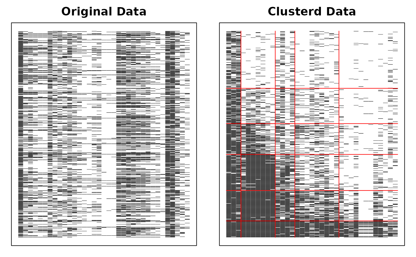
Biclustering.RdPerforms biclustering, ranklustering, or their confirmatory variants on binary response data. These methods simultaneously cluster both examinees and items into homogeneous groups (or ordered ranks for ranklustering). The analysis reveals latent structures and patterns in the data by creating a matrix with rows and columns arranged to highlight block structures.
Usage
Biclustering(U, ...)

# Default S3 method
Biclustering(U, na = NULL, Z = NULL, w = NULL, ...)

# S3 method for class 'binary'
Biclustering(
  U,
  ncls = 2,
  nfld = 2,
  method = "B",
  estimation = "isotonic",
  conf = NULL,
  conf_class = NULL,
  mic = FALSE,
  maxiter = 1000,
  verbose = FALSE,
  beta1 = 1,
  beta2 = 1,
  ...
)

# S3 method for class 'nominal'
Biclustering(
  U,
  ncls = 2,
  nfld = 2,
  conf = NULL,
  conf_class = NULL,
  mic = FALSE,
  maxiter = 1000,
  verbose = FALSE,
  alpha = 1,
  ...
)

# S3 method for class 'ordinal'
Biclustering(
  U,
  ncls = 2,
  nfld = 2,
  method = "B",
  estimation = "isotonic",
  conf = NULL,
  conf_class = NULL,
  mic = FALSE,
  maxiter = 1000,
  verbose = FALSE,
  alpha = 1,
  init = c("auto", "quantile", "ward", "legacy"),
  nstart = 10,
  seed = 1,
  ...
)

# S3 method for class 'rated'
Biclustering(
  U,
  ncls = 2,
  nfld = 2,
  method = "R",
  conf = NULL,
  conf_class = NULL,
  maxiter = 1000,
  verbose = FALSE,
  alpha = 1,
  ...
)
Arguments
- U
Either an object of class "exametrika" or raw data. When raw data is given, it is converted to the exametrika class with the
dataFormatfunction.- ...
Additional arguments passed to specific methods.
- na
Values to be treated as missing values.
- Z
Missing indicator matrix of type matrix or data.frame. Values of 1 indicate observed responses, while 0 indicates missing data.
- w
Item weight vector specifying the relative importance of each item.
- ncls
Number of latent classes/ranks to identify (between 2 and 20).
- nfld
Number of latent fields (item clusters) to identify.
- method
Analysis method to use (character string):
"B" or "Biclustering": Standard biclustering (default for binary and ordinal data)
"R" or "Ranklustering": Ranklustering with ordered class structure (default for rated data, where classes are sorted by correct response rate)
- estimation
Estimation method for the Field Reference Profiles under Ranklustering (
method = "R"); ignored for plain Biclustering, whose classes are unordered:"isotonic": order-restricted estimation, imposing the rank ordering directly in the M-step (default). For binary data this is a weighted pool-adjacent-violators step, which under the default flat prior is the exact order-restricted MLE (Ayer et al. 1955); for ordinal data it is the stochastic-order-restricted multinomial MAP solved by the Fenchel-dual algorithm (El Barmi & Dykstra 1994).
"GTM": the original filter-based smoothing of Shojima (2012).
- conf
Confirmatory parameter for pre-specified field assignments. Can be either:
A vector with items and corresponding fields in sequence
A field membership profile matrix (items x fields) with 0/1 values
NULL (default) for exploratory analysis where field memberships are estimated
- conf_class
Confirmatory parameter for pre-specified class assignments on the respondent side. Mirrors
confbut operates on classes. Can be:A vector with respondents and corresponding class indices
A class membership profile matrix (respondents × classes) with 0/1 values
NULL (default) for exploratory class estimation When supplied, class memberships are held fixed during EM. For Ranklustering (
method = "R"), the neighbour-smoothing step is skipped because smoothing pre-specified labels would defeat the purpose of fixing them.
- mic
Logical; if TRUE, forces Field Reference Profiles to be monotonically increasing. Default is FALSE.
- maxiter
Maximum number of EM algorithm iterations. Default is 1000.
- verbose
Logical; if TRUE, displays progress during estimation. Default is FALSE.
- beta1
Beta distribution parameter 1 for prior density of field reference matrix. Default is 1.
- beta2
Beta distribution parameter 2 for prior density of field reference matrix. Default is 1.
- alpha
Dirichlet distribution concentration parameter for prior density of field reference probabilities. Default is 1.
- init
Starting values of the EM (character string). The EM is deterministic but converges to a local optimum, so the start matters:
"auto" (default): run from both "quantile" and "ward" and keep the fit with the larger ELBO
"quantile": classes from equal-count bins of the respondent score
"ward": classes from Ward clustering of the respondent score (does not assume equal class sizes)
"legacy": the start used up to 2.2.0 (fields by item median, a common class ladder); reproduces earlier results
In "quantile" and "ward" the fields start from a Ward clustering of the items' class-mean profiles; with
confthe fields are the given ones, and withconf_classthe classes are the given ones (a single start).- nstart
Number of random starts added to
init = "auto"(ignored for the otherinitvalues and withconf_class). The classes of a random start are random; its fields areconfif given, and otherwise those of the "quantile" start for half of the starts and random for the other half. Every random start is first run for 100 EM cycles and only the best 3 by ELBO are run to convergence. Set 0 for the two data-based starts only; raise it (e.g. 50 or 100) for data with many local optima, which costs time roughly in proportion.- seed
Seed of the random starts. The random number stream of the session is left untouched, so the fit is reproducible.
Value
An object of class "exametrika" and "Biclustering" containing:
- model
Model type indicator (1 for biclustering, 2 for ranklustering)
- msg
A character string indicating the model type.
- mic
Logical value indicating whether monotonicity constraint was applied
- testlength
Number of items in the test
- nobs
Number of examinees in the dataset
- n_class
Number of latent classes/ranks specified
- n_field
Number of latent fields specified
- n_cycle
Number of EM iterations performed
- converge
Logical value indicating whether the algorithm converged within maxiter iterations
- LFD
Latent Field Distribution - counts of items assigned to each field
- LRD/LCD
Latent Rank/Class Distribution - counts of examinees assigned to each class/rank
- FRP
Field Reference Profile matrix - probability of correct response for each field-class combination
- CategoryShift
Nominal and ordinal data only. The amount added to every category code to make the codes start at 1; used by
predict.exametrika().- FRPIndex
Field Reference Profile indices (Kumagai, 2007) — data.frame with 6 columns:
- Alpha
Maximum-slope location: class transition where the largest increase occurs
- A
Maximum slope: largest consecutive-class difference in the profile
- Beta
Location parameter: class whose FRP value is closest to 0.5
- B
FRP value at the Beta position
- Gamma
Non-monotonicity ratio: proportion of class transitions that decrease
- C
Monotonicity violation: sum of negative consecutive-class differences (C=0 means perfectly monotone)
For binary data, computed directly from the FRP matrix (correct response rates). For ordinal data, computed from normalized expected scores: (E[score]-1)/(maxQ-1), which maps expected scores from [1, maxQ] to [0, 1] for comparability with the binary case. Not computed for nominal data (no natural category ordering).
- TRP
Test Reference Profile - expected score for examinees in each class/rank. For ordinal data it is computed from the model since 2.2.0 (the sum over fields of field size times the field expected score), as for binary data, so SOAC and WOAC judge the estimates.
- TRP_empirical
Ordinal data only. The same profile from the data: the mean observed score of the members of each class/rank, summed over fields. Its departure from
TRPshows how far the model is from the data. Since 2.2.0.- CMD/RMD
Class/Rank Membership Distribution - sum of membership probabilities across examinees
- FieldMembership
Matrix showing the probabilities of each item belonging to each field
- ClassMembership
Matrix showing the probabilities of each examinee belonging to each class/rank
- SmoothedMembership
Matrix of smoothed class membership probabilities after filtering
- FieldEstimated
Vector of the most likely field assignments for each item
- ClassEstimated
Vector of the most likely class/rank assignments for each examinee
- Students
Data frame containing membership probabilities and classification information for each examinee
- FieldAnalysis
Matrix showing field analysis results with item-level information
- TestFitIndices
Model fit indices for evaluating the quality of the clustering solution
- log_lik
Log-likelihood the fit indices are built on. For binary data this is the expected log-likelihood of the reference implementation; for nominal and ordinal data it is the evidence lower bound (
elbo) since 2.2.0. Rated data report the binary layer here and the nominal layer with the suffix_nominal.- elbo
Evidence lower bound of the observed-data log-likelihood under the posterior memberships the EM produced. Exact (equal to the observed-data log-likelihood) for a one-mode model; a lower bound for biclustering, where the respondent and item posteriors are taken independent. Since 2.2.0.
- log_lik_marginal
Observed-data log-likelihood of the respondent-side mixture with the items fixed at their MAP field assignment. Equal to
elbofor a one-mode model.- entropy
Posterior entropy of the memberships (named:
class, andfieldfor biclustering).elbominus this is the expected complete-data log-likelihood.- ICL
Integrated completed likelihood criterion (Biernacki, Celeux and Govaert, 2000) in its BIC-type approximation, on the same scale as AIC and BIC (-2 log scale, smaller is better).
- init, init_selected, init_elbo
Ordinal data only. The
initrequested, the start whose fit is returned, and the ELBO reached from each start that was run. Since 2.2.0.- SOACflg
Logical flag indicating whether Strongly Ordinal Alignment Condition is satisfied
- WOACflg
Logical flag indicating whether Weakly Ordinal Alignment Condition is satisfied
Details
Biclustering simultaneously clusters both rows (examinees) and columns (items) of a data matrix. Unlike traditional clustering that groups either rows or columns, biclustering identifies submatrices with similar patterns. Ranklustering is a variant that imposes an ordinal structure on the classes, making it suitable for proficiency scaling.
The algorithm uses an Expectation-Maximization approach to iteratively estimate:
Field membership of items (which items belong to which fields)
Class/rank membership of examinees (which examinees belong to which classes)
Field Reference Profiles (probability patterns for each field-class combination)
The confirmatory option allows for pre-specified field assignments, which is useful when there is prior knowledge about item groupings or for testing hypothesized structures.
References
Shojima, K. (2012). Biclustering of binary data matrices using bilinear models. Behaviormetrika, 39(2), 161-178.
Examples
# \donttest{
# Perform Biclustering with Binary method (B)
# Analyze data with 5 fields and 6 classes
result.Bi <- Biclustering(J35S515, nfld = 5, ncls = 6, method = "B")
# Perform Biclustering with Rank method (R)
# Store results for further analysis and visualization
result.Rank <- Biclustering(J35S515, nfld = 5, ncls = 6, method = "R")
# Display the Bicluster Reference Matrix (BRM) as a heatmap
plot(result.Rank, type = "Array")
 # Plot Field Reference Profiles (FRP) in a 2x3 grid
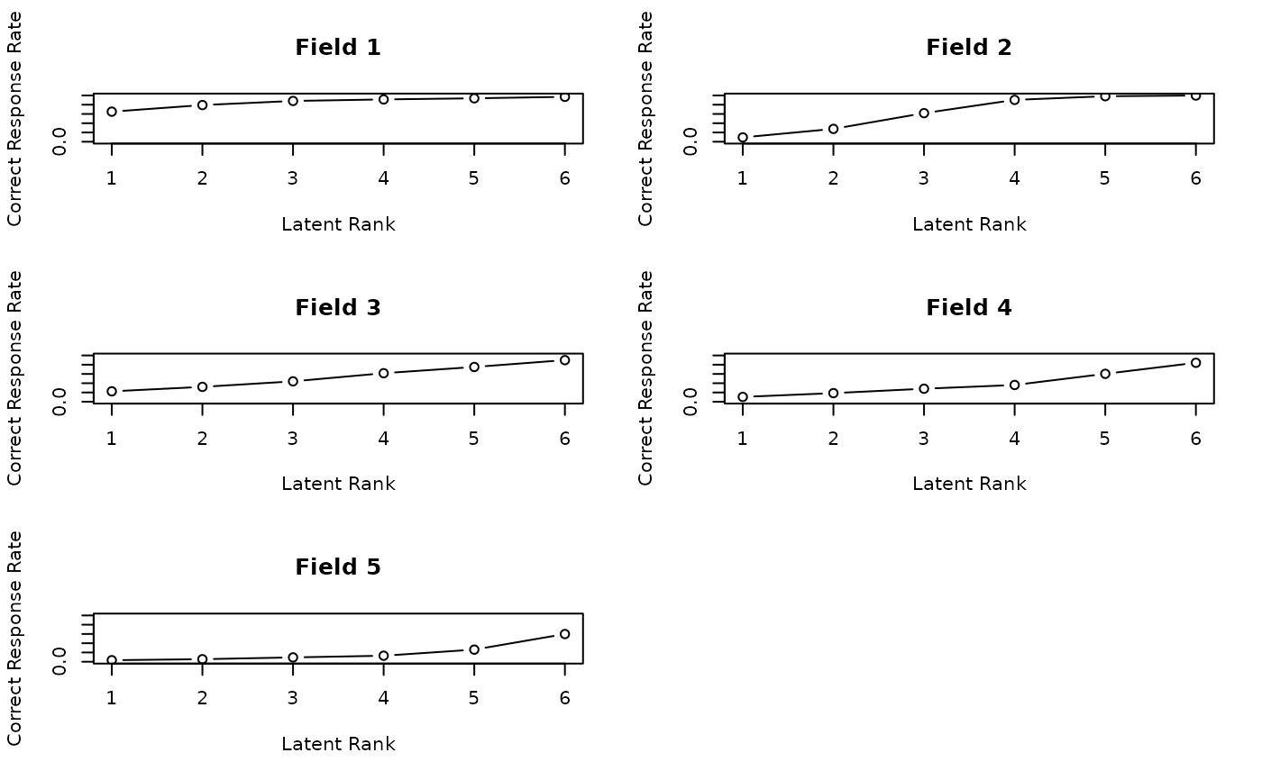
# Shows the probability patterns for each field
plot(result.Rank, type = "FRP", nc = 2, nr = 3)
# Plot Field Reference Profiles (FRP) in a 2x3 grid
# Shows the probability patterns for each field
plot(result.Rank, type = "FRP", nc = 2, nr = 3)
 # Plot Rank Membership Profiles (RMP) for students 1-9 in a 3x3 grid
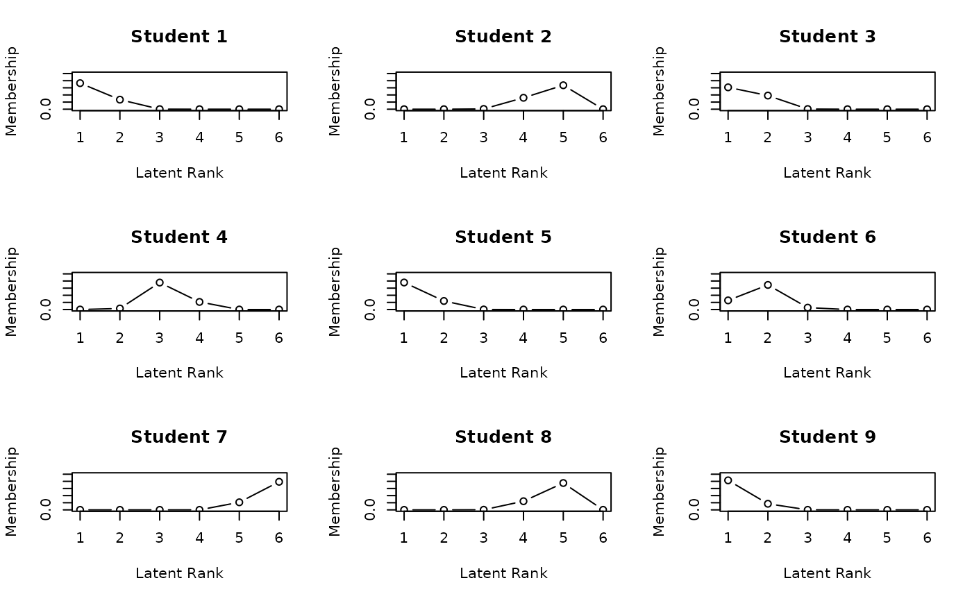
# Shows posterior probability distribution of rank membership
plot(result.Rank, type = "RMP", students = 1:9, nc = 3, nr = 3)
# Plot Rank Membership Profiles (RMP) for students 1-9 in a 3x3 grid
# Shows posterior probability distribution of rank membership
plot(result.Rank, type = "RMP", students = 1:9, nc = 3, nr = 3)
 # Example of confirmatory analysis with pre-specified fields
# Assign items 1-10 to field 1, 11-20 to field 2, etc.
field_assignments <- c(rep(1, 10), rep(2, 10), rep(3, 15))
result.Conf <- Biclustering(J35S515, nfld = 3, ncls = 5, conf = field_assignments)
# }
# \donttest{
# Perform Biclustering for nominal sample data()
# Analyze data with 5 fields and 6 classes
result.Bi <- Biclustering(J35S515, nfld = 5, ncls = 6, method = "B")
# }
# \donttest{
# Perform Biclustering for rated sample data
# Analyze data with 5 fields and 6 classes
result.Bi <- Biclustering(J35S5000, nfld = 5, ncls = 6, method = "R")
# }
# Example of confirmatory analysis with pre-specified fields
# Assign items 1-10 to field 1, 11-20 to field 2, etc.
field_assignments <- c(rep(1, 10), rep(2, 10), rep(3, 15))
result.Conf <- Biclustering(J35S515, nfld = 3, ncls = 5, conf = field_assignments)
# }
# \donttest{
# Perform Biclustering for nominal sample data()
# Analyze data with 5 fields and 6 classes
result.Bi <- Biclustering(J35S515, nfld = 5, ncls = 6, method = "B")
# }
# \donttest{
# Perform Biclustering for rated sample data
# Analyze data with 5 fields and 6 classes
result.Bi <- Biclustering(J35S5000, nfld = 5, ncls = 6, method = "R")
# }