Latent Class Analysis

Performs Latent Class Analysis (LCA) on binary response data using the Expectation-Maximization (EM) algorithm. LCA identifies unobserved (latent) subgroups of examinees with similar response patterns, and estimates both the class characteristics and individual membership probabilities.

Usage

LCA(U, ...)

# Default S3 method
LCA(U, na = NULL, Z = NULL, w = NULL, ...)

# S3 method for class 'binary'
LCA(
  U,
  ncls = 2,
  na = NULL,
  Z = NULL,
  w = NULL,
  maxiter = 1000,
  verbose = FALSE,
  beta1 = 1,
  beta2 = 1,
  conf = NULL,
  ...
)

# S3 method for class 'nominal'
LCA(
  U,
  ncls = 2,
  na = NULL,
  Z = NULL,
  w = NULL,
  maxiter = 1000,
  verbose = FALSE,
  alpha = 1,
  ...
)

# S3 method for class 'rated'
LCA(
  U,
  ncls = 2,
  na = NULL,
  Z = NULL,
  w = NULL,
  maxiter = 1000,
  verbose = FALSE,
  alpha = 1,
  ...
)

Arguments

U

Either an object of class "exametrika" or raw data. When raw data is given, it is converted to the exametrika class with the dataFormat function.

...

Additional arguments passed to specific methods.

na

Values to be treated as missing values.

Z

Missing indicator matrix of type matrix or data.frame. Values of 1 indicate observed responses, while 0 indicates missing data.

w

Item weight vector specifying the relative importance of each item.

ncls

Number of latent classes to identify (between 2 and 20). Default is 2.

maxiter

Maximum number of EM algorithm iterations. Default is 1000.

verbose

Logical; if TRUE, displays progress during estimation. Default is FALSE.

beta1

Beta distribution parameter 1 for prior density of class reference matrix. Default is 1.

beta2

Beta distribution parameter 2 for prior density of class reference matrix. Default is 1.

conf

Confirmatory IRP matrix (items x ncls) for test equating. Same format as the IRP output. Non-NA values are fixed throughout estimation, NA values are freely estimated. Fixed values must be in the open interval (0, 1). When row names are present, items are matched by label; otherwise by position. Default is NULL (fully exploratory).

alpha

Dirichlet prior parameter for the category profiles (nominal data only). Default 1, which leaves the M-step at the plain multinomial MLE.

Value

An object of class "exametrika" and "LCA" containing:

msg

A character string indicating the model type.

testlength

Length of the test (number of items).

nobs

Sample size (number of rows in the dataset).

n_class

Number of latent classes specified.

n_cycle

Number of EM algorithm iterations performed.

converge

Logical value indicating whether the algorithm converged within maxiter iterations

TRP

Test Reference Profile vector showing expected scores for each latent class. Calculated as the column sum of the estimated class reference matrix.

LCD

Latent Class Distribution vector showing the number of examinees assigned to each latent class.

CMD

Class Membership Distribution vector showing the sum of membership probabilities for each latent class.

Students

Class Membership Profile matrix showing the posterior probability of each examinee belonging to each latent class. The last column ("Estimate") indicates the most likely class assignment.

IRP

Item Reference Profile matrix where each row represents an item and each column represents a latent class. Values indicate the probability of a correct response for members of that class.

ItemFitIndices

Fit indices for each item. See also ItemFit.

TestFitIndices

Overall fit indices for the test. See also TestFit.

Details

Latent Class Analysis is a statistical method for identifying unobserved subgroups within a population based on observed response patterns. It assumes that examinees belong to one of several distinct latent classes, and that the probability of a correct response to each item depends on class membership.

The algorithm proceeds by:

1. Initializing class reference probabilities

2. Computing posterior class membership probabilities for each examinee (E-step)

3. Re-estimating class reference probabilities based on these memberships (M-step)

4. Iterating until convergence or reaching the maximum number of iterations

Unlike Item Response Theory (IRT), LCA treats latent variables as categorical rather than continuous, identifying distinct profiles rather than positions on a continuum.

For nominal data the model is a finite mixture of product-multinomial distributions: every latent class carries an independent category distribution for each item, and no ordering is imposed on the classes or on the categories. Category counts may differ across items.

Ordered rating data is routed to this method as well, because unordered latent classes give the category order nothing to attach to. Use LRA when the ordering should be respected.

No benchmark (saturated) model is fitted, for the same reason as in Biclustering.nominal: with many items and categories nearly every response pattern is unique, so the saturated log-likelihood is not informative. Only AIC, BIC and CAIC are reported; the chi-square based indices are NA.

For rated data (multiple-choice items with a key) the estimation is the nominal one — LCA.rated calls LCA.nominal internally — and the key is used afterwards to recover the quantities that need a notion of a correct answer. The Item Reference Profile is the model-implied probability of the keyed category, IRP[j, c] = rho[j, CA[j] | c], and the Test Reference Profile is its weighted item sum. Unlike Biclustering on rated data, the classes are not sorted by correct response rate: latent classes carry no order, and sorting them would suggest one.

Two layers of fit are reported. TestFitIndices is the binary layer, built from correct/incorrect responses under the class-membership-weighted correct probabilities, so it carries the usual chi-square based indices and is comparable with binary LCA. TestFitIndicesNominal is the nominal layer taken from the internal fit, with AIC/BIC/CAIC only. The full category probabilities stay in ICRP for distractor analysis.

References

Goodman, L. A. (1974). Exploratory latent structure analysis using both identifiable and unidentifiable models. Biometrika, 61(2), 215-231.

Lazarsfeld, P. F., & Henry, N. W. (1968). Latent structure analysis. Boston: Houghton Mifflin.

Examples

# \donttest{
# Fit a Latent Class Analysis model with 5 classes to the sample dataset
result.LCA <- LCA(J15S500, ncls = 5)

# Display the first few rows of student class membership probabilities
head(result.LCA$Students)
#>            Membership 1 Membership 2 Membership 3 Membership 4 Membership 5
#> Student001 0.7285244374  0.012211535  0.226232540 3.303149e-02 3.055593e-12
#> Student002 0.0220645036  0.086986302  0.830839343 6.010974e-02 1.074954e-07
#> Student003 0.0170578933  0.054109896  0.879752304 2.100872e-02 2.807118e-02
#> Student004 0.0010508039  0.223175413  0.203820488 3.286491e-01 2.433042e-01
#> Student005 0.9407961670  0.053321705  0.004873703 1.808344e-08 1.008407e-03
#> Student006 0.0002372397  0.002528968  0.029747250 8.551046e-01 1.123819e-01
#>            Estimate
#> Student001        1
#> Student002        3
#> Student003        3
#> Student004        4
#> Student005        1
#> Student006        4

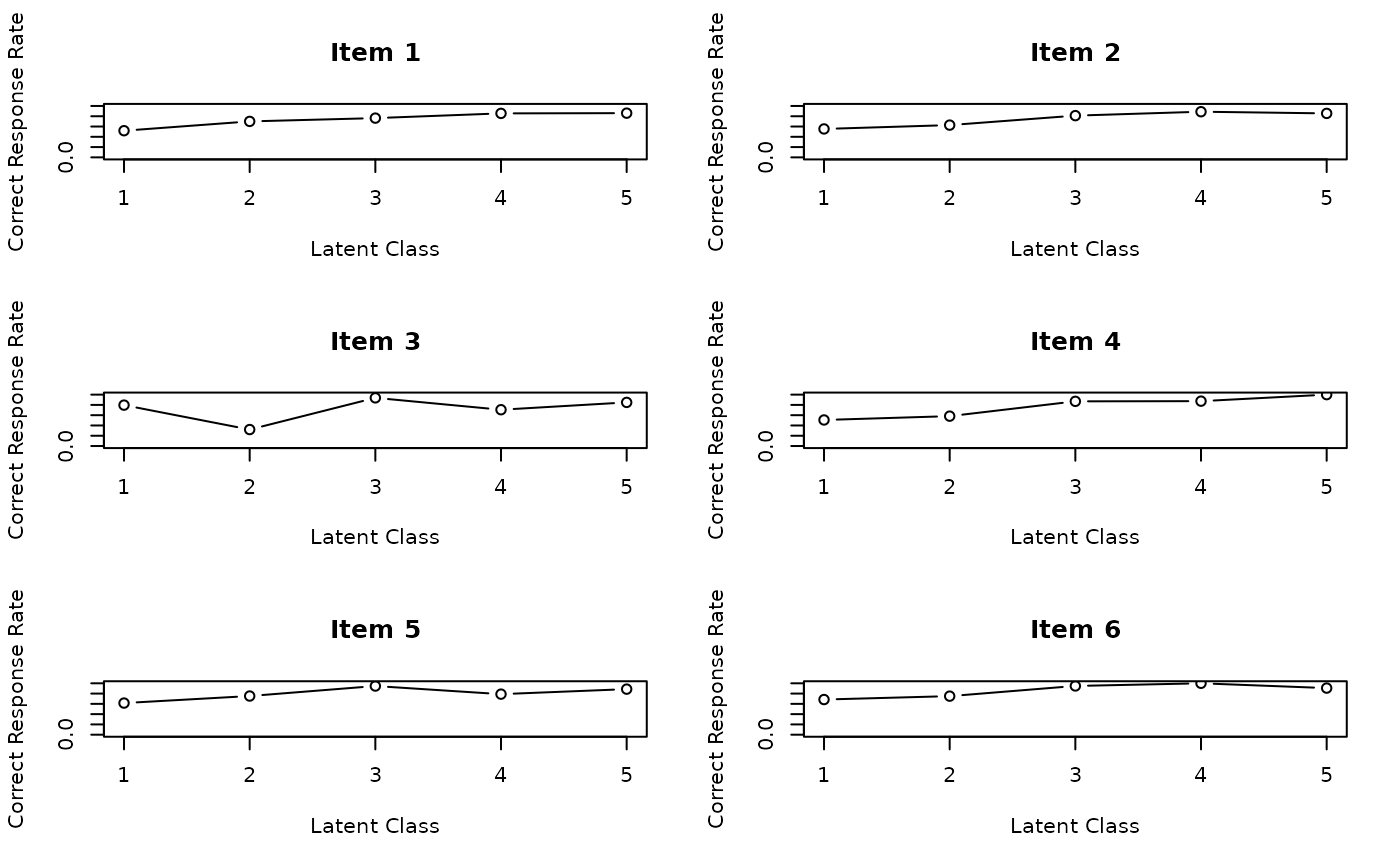
# Plot Item Response Profiles (IRP) for items 1-6 in a 2x3 grid
# Shows probability of correct response for each item across classes
plot(result.LCA, type = "IRP", items = 1:6, nc = 2, nr = 3)


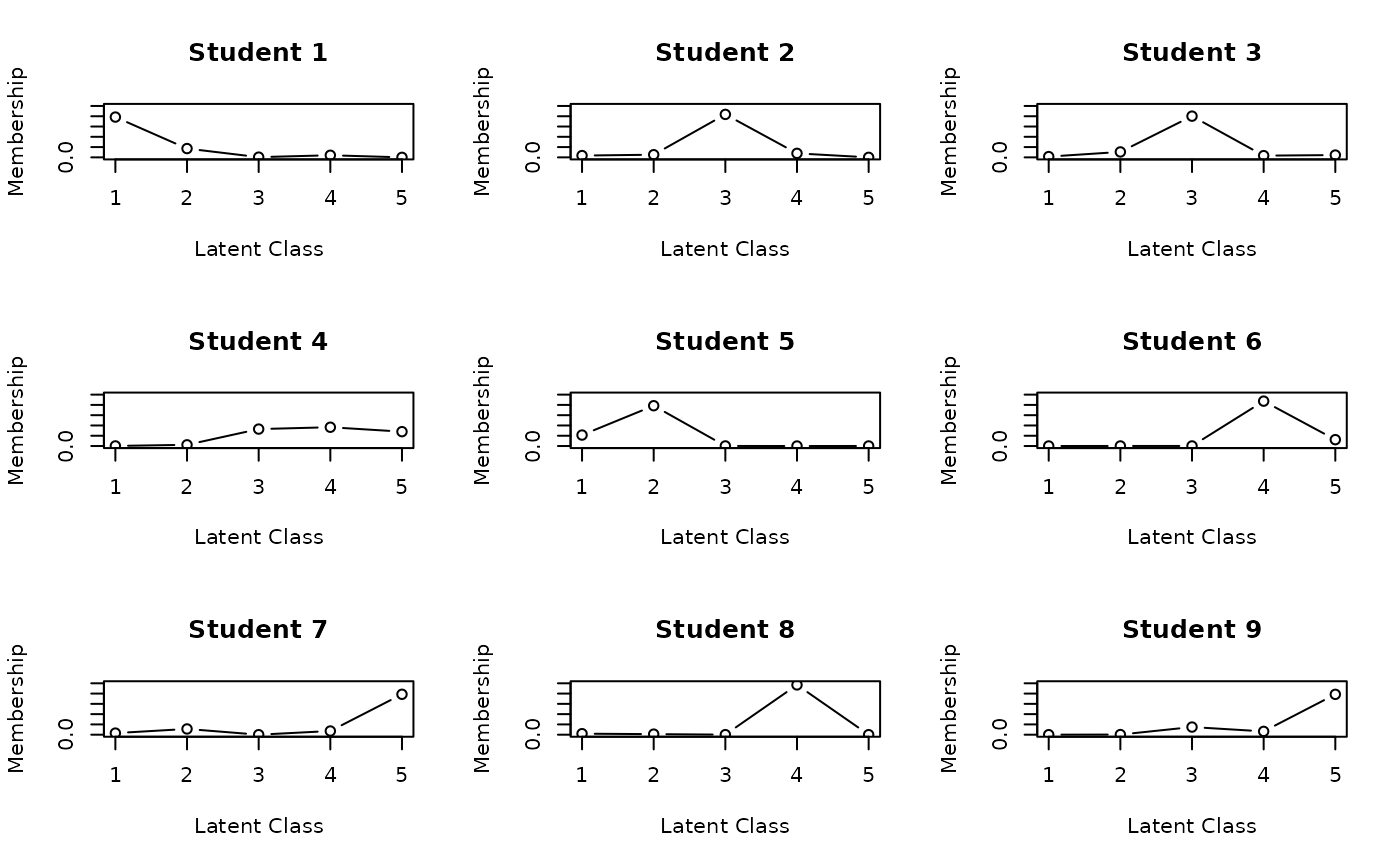
# Plot Class Membership Probabilities (CMP) for students 1-9 in a 3x3 grid
# Shows probability distribution of class membership for each student
plot(result.LCA, type = "CMP", students = 1:9, nc = 3, nr = 3)


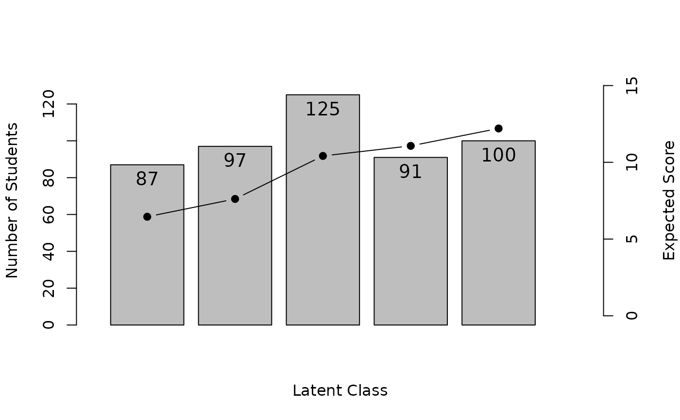
# Plot Test Response Profile (TRP) showing expected scores for each class
plot(result.LCA, type = "TRP")


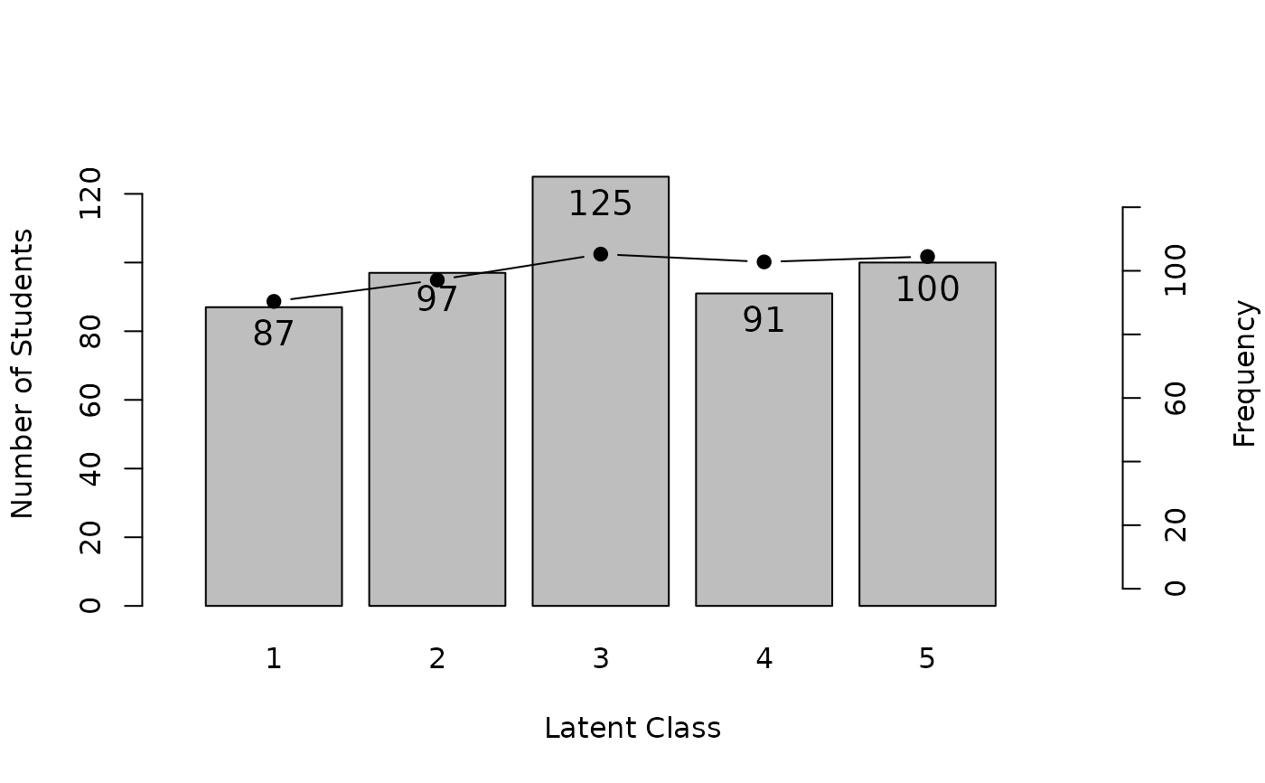
# Plot Latent Class Distribution (LCD) showing class sizes
plot(result.LCA, type = "LCD")


# Compare models with different numbers of classes
# (In practice, you might try more class counts)
lca2 <- LCA(J15S500, ncls = 2)
lca3 <- LCA(J15S500, ncls = 3)
lca4 <- LCA(J15S500, ncls = 4)
lca5 <- LCA(J15S500, ncls = 5)

# Compare BIC values to select optimal number of classes
# (Lower BIC indicates better fit)
data.frame(
  Classes = 2:5,
  BIC = c(
    lca2$TestFitIndices$BIC,
    lca3$TestFitIndices$BIC,
    lca4$TestFitIndices$BIC,
    lca5$TestFitIndices$BIC
  )
)
#>   Classes       BIC
#> 1       2 -346.3585
#> 2       3 -464.5868
#> 3       4 -609.6852
#> 4       5 -655.1747
# }