確率モデルは面白い
7scientist
## データの準備
X <- c(-27.020,3.570,8.191,9.808,9.603,9.945,10.056)
sc7 <- list(N=NROW(X),X=X)
## モデルコンパイル
model <- stan_model("SevenScientist.stan")
## data{
##   int<lower=0> N;
##   real X[N];
## }
##
## parameters{
##   real mu;
##   real<lower=0> sig[N];
## }
##
## model{
##   for(n in 1:N){
##     //likelihood
##     X[n] ~ normal(mu,sig[n]);
##     //prior
##     sig[n] ~ inv_gamma(0.0001,0.0001);
##   }
##   // prior
##   mu ~ normal(0,1000);
## }
## 推定
fit <- sampling(model,sc7,iter=10000)
## Warning: There were 7154 divergent transitions after warmup. Increasing adapt_delta above 0.8 may help. See
## http://mc-stan.org/misc/warnings.html#divergent-transitions-after-warmup
## Warning: Examine the pairs() plot to diagnose sampling problems
##  表示
fit
## Inference for Stan model: SevenScientist.
## 4 chains, each with iter=10000; warmup=5000; thin=1;
## post-warmup draws per chain=5000, total post-warmup draws=20000.
##
##          mean se_mean     sd  2.5%   25%   50%    75%  97.5% n_eff Rhat
## mu       9.90    0.01   0.11  9.60  9.81  9.94   9.95  10.06   104 1.03
## sig[1] 154.21   13.63 906.95 17.49 32.33 51.92 107.89 576.71  4426 1.00
## sig[2]  34.45    6.60 439.63  2.94  5.80 10.01  20.97 153.57  4438 1.00
## sig[3]   7.66    0.82  53.58  0.77  1.55  2.79   6.32  25.70  4264 1.00
## sig[4]   0.43    0.04   3.28  0.00  0.06  0.15   0.29   1.97  7303 1.00
## sig[5]   2.38    0.78  62.10  0.03  0.25  0.41   0.75   6.07  6311 1.00
## sig[6]   0.52    0.09   8.72  0.00  0.00  0.08   0.23   1.99  9369 1.00
## sig[7]   1.13    0.31  34.71  0.00  0.08  0.19   0.48   3.62 12485 1.00
## lp__    -3.26    0.39   2.92 -9.71 -5.25 -2.94  -0.86   0.90    55 1.09
##
## Samples were drawn using NUTS(diag_e) at Mon Sep  3 19:35:11 2018.
## For each parameter, n_eff is a crude measure of effective sample size,
## and Rhat is the potential scale reduction factor on split chains (at
## convergence, Rhat=1).
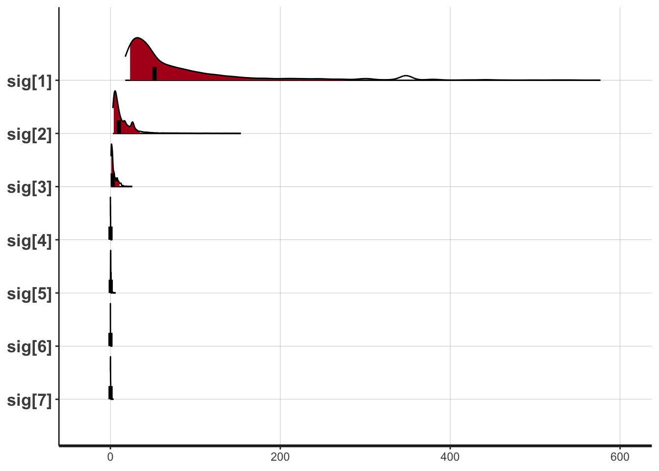
## 描画
plot(fit,pars=c("sig[1]","sig[2]","sig[3]","sig[4]",
                "sig[5]","sig[6]","sig[7]"),show_density=T)
## ci_level: 0.8 (80% intervals)
## outer_level: 0.95 (95% intervals)
打ち切りデータ
## データの準備
nfails     <- 949
n          <- 50    # Number of questions
datasasoon <- list(nF=nfails,N=n)
## モデルコンパイル
sasoon <- stan_model("censored.stan")
## data{
##   int<lower=0> nF; // number of failes
##   int<lower=0> N;  // number of questions
## }
##
## parameters{
##   real<lower=0.25,upper=1> theta;
## }
##
## model{
##   30 ~ binomial(N,theta);
##   target += nF * (log(binomial_cdf(25,N,theta) - binomial_cdf(14,N,theta)));
## }
fit <- sampling(sasoon,datasasoon)
fit
## Inference for Stan model: censored.
## 4 chains, each with iter=2000; warmup=1000; thin=1;
## post-warmup draws per chain=1000, total post-warmup draws=4000.
##
##          mean se_mean   sd    2.5%     25%     50%    75%   97.5% n_eff
## theta    0.40    0.00 0.00    0.39    0.40    0.40    0.4    0.41  1228
## lp__  -152.25    0.02 0.69 -154.19 -152.42 -151.98 -151.8 -151.75  1291
##       Rhat
## theta    1
## lp__     1
##
## Samples were drawn using NUTS(diag_e) at Mon Sep  3 19:35:15 2018.
## For each parameter, n_eff is a crude measure of effective sample size,
## and Rhat is the potential scale reduction factor on split chains (at
## convergence, Rhat=1).
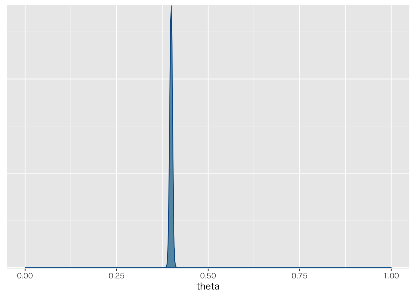
fit %>% as.array %>%
  bayesplot::mcmc_dens(pars="theta") + xlim(0,1)
## Scale for 'x' is already present. Adding another scale for 'x', which
## will replace the existing scale.
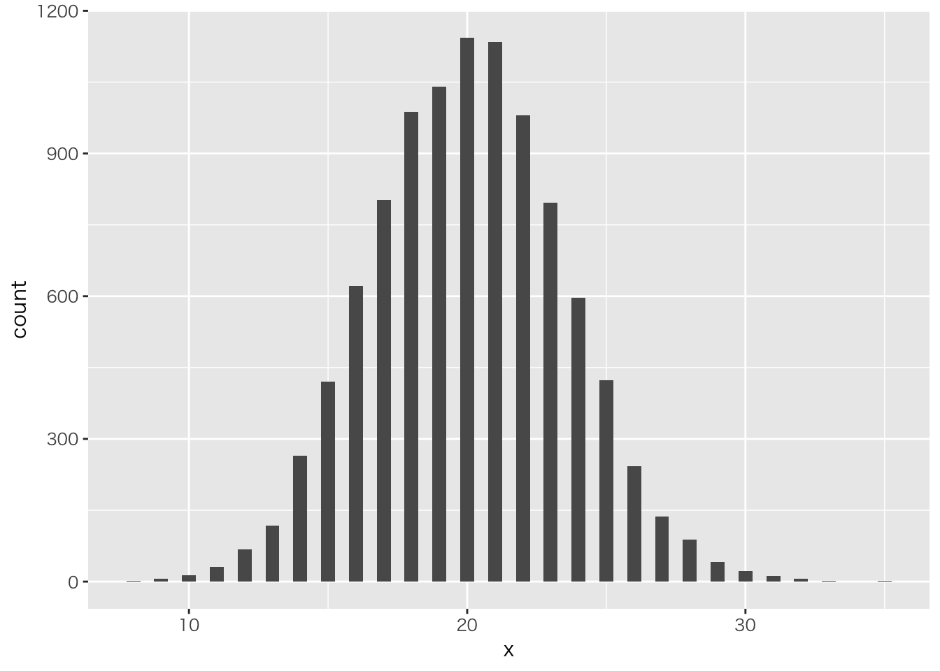
二項分布を確認しておこう
二項分布の例
theta <- 0.4
Ntrial <- 50
size <- 10000
data.frame(x=rbinom(size,Ntrial,theta)) %>%
  ggplot(aes(x=x))+geom_histogram(binwidth = 0.5)
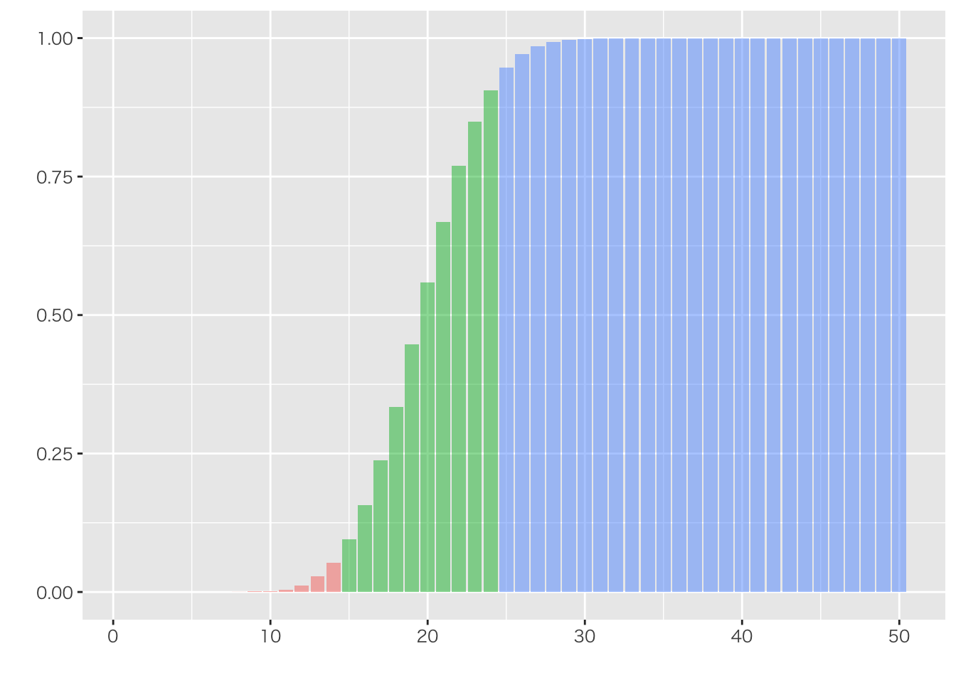
今回の例を乱数で作ってみる
### 仮にtheta=0.4とする
N <- 10000
data.frame(X=rbinom(N,50,0.4)) %>%
  table() %>% data.frame() %>%
  rename(tbl=1) %>% mutate(tbl=as.numeric(levels(tbl)[tbl])) %>%
  right_join(.,data.frame(tbl=1:50)) %>%
  mutate(Freq=replace_na(Freq,0)) %>%
  mutate(Cum = cumsum(Freq)/N) %>%
  mutate(COL = ifelse(tbl<15,1,ifelse(tbl<25,2,3))) %>%
  ggplot(aes(x=tbl,y=Cum,fill=as.factor(COL))) +
  geom_bar(stat="identity",alpha=0.5) +
  xlab("")+ylab("")+ theme(legend.position = "none")
## Joining, by = "tbl"
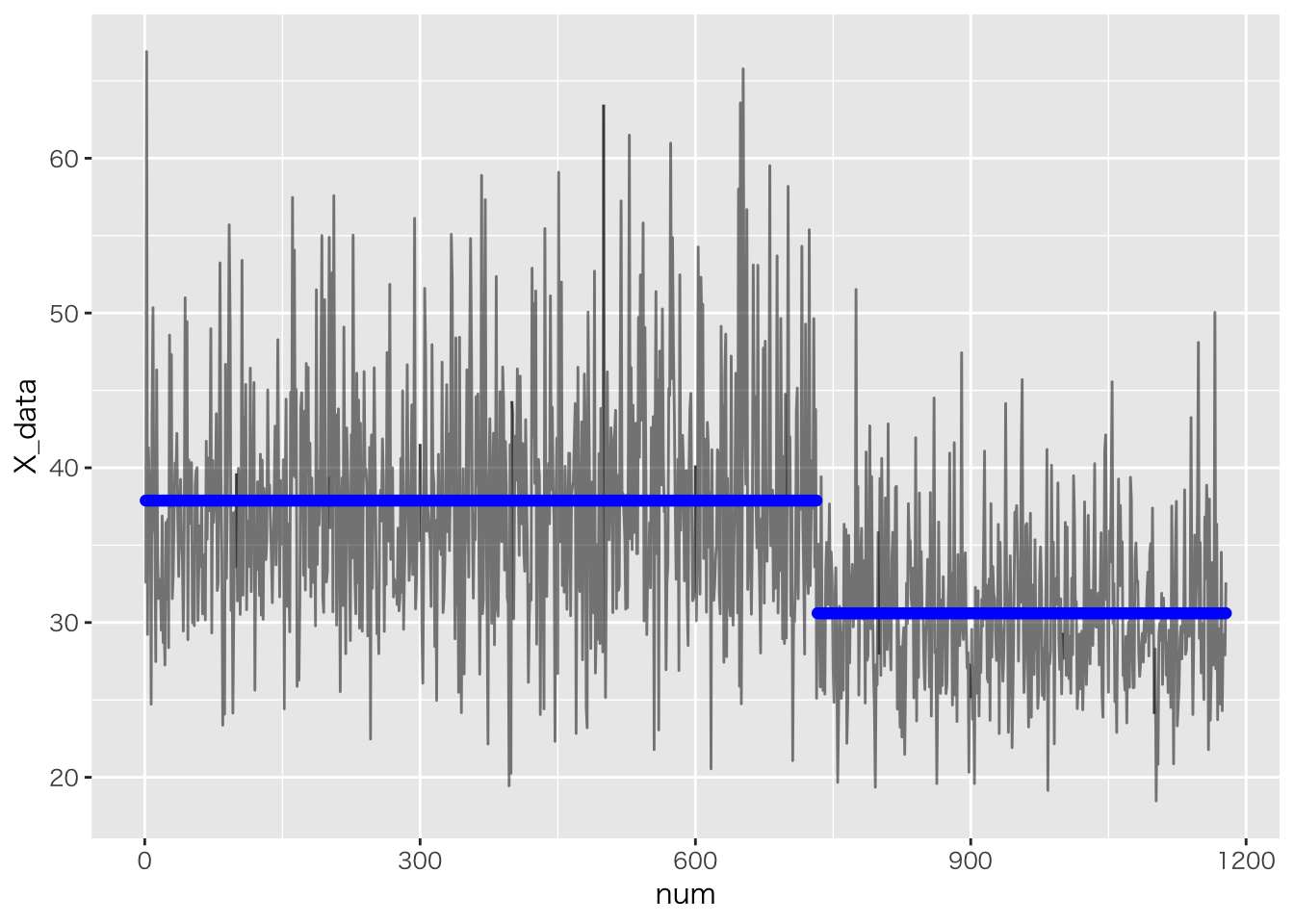
変化点の検出
c <- scan("changepointdata.txt")
n <- length(c)
t <- 1:n
datapoints <- list(C=c,N=n,Time=t)
ChangeDetection <- stan_model("ChangeDetection.stan")
## data{
##   int<lower=0> N;
##   int<lower=0> Time[N];
##   real C[N];
## }
##
## parameters{
##   vector<lower=0>[2] mu;
##   real<lower=0> sigma;
##   real<lower=0,upper=N> tau;
## }
##
##
## model{
##   //prior
##   mu[1] ~ normal(0,1000);
##   mu[2] ~ normal(0,1000);
##   sigma ~ cauchy(0,5);
##
##   //likelihood
##   for(n in 1:N){
##     if(Time[n]> tau){
##       C[n] ~ normal(mu[2],sigma);
##     } else {
##       C[n] ~ normal(mu[1],sigma);
##     }
##   }
##
##   tau ~ uniform(0,N);
## }
fit <- sampling(ChangeDetection,datapoints)
## Warning: There were 3994 transitions after warmup that exceeded the maximum treedepth. Increase max_treedepth above 10. See
## http://mc-stan.org/misc/warnings.html#maximum-treedepth-exceeded
## Warning: Examine the pairs() plot to diagnose sampling problems
print(fit)
## Inference for Stan model: ChangeDetection.
## 4 chains, each with iter=2000; warmup=1000; thin=1;
## post-warmup draws per chain=1000, total post-warmup draws=4000.
##
##           mean se_mean   sd     2.5%      25%      50%      75%    97.5%
## mu[1]    37.88    0.03 0.27    37.37    37.70    37.88    38.06    38.41
## mu[2]    30.60    0.02 0.30    30.00    30.39    30.60    30.81    31.18
## sigma     6.84    0.01 0.13     6.58     6.75     6.84     6.93     7.10
## tau     732.08    0.12 1.93   729.08   731.08   731.70   733.01   737.12
## lp__  -2841.63    0.08 1.47 -2845.05 -2842.39 -2841.43 -2840.58 -2839.47
##       n_eff Rhat
## mu[1]   109 1.03
## mu[2]   177 1.02
## sigma    93 1.01
## tau     241 1.01
## lp__    333 1.01
##
## Samples were drawn using NUTS(diag_e) at Mon Sep  3 19:40:18 2018.
## For each parameter, n_eff is a crude measure of effective sample size,
## and Rhat is the potential scale reduction factor on split chains (at
## convergence, Rhat=1).
可視化
df <- transform(c)
Ms <- rstan::get_posterior_mean(fit,pars="mu")[,5]
point <- round(apply(as.matrix(rstan::extract(fit,pars="tau")$tau),2,median))
df$Mu <- c(rep(Ms[1],point),rep(Ms[2],n-point))
df %>% dplyr::mutate(num=row_number()) %>% ggplot(aes(x=num,y=X_data))+geom_line(alpha=0.5)+
  geom_point(aes(y=Mu),color="blue")
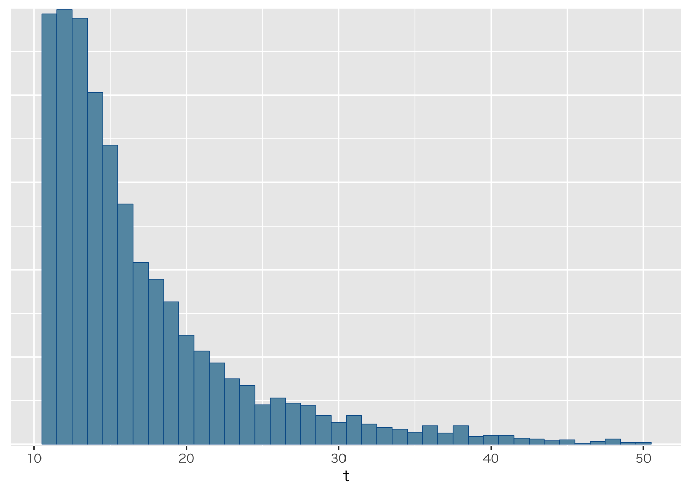
飛行機を再捕獲する
x <- 10 # number of captures
k <- 4  # number of recaptures from n
n <- 5  # size of second sample
tmax <- 50 # maximum population size
datastan <- list(X=x,N=n,K=k,TMax=tmax)
planeModel <- stan_model("plane.stan")
## data{
##   int<lower=0> X; //第一標本サイズ
##   int<lower=0> N; //第二標本サイズ
##   int<lower=0,upper=N> K; //再捕獲した数
##   int<lower=X> TMax; // ありえそうな最大数
## }
##
## transformed data{
##   int<lower=X> tmin; //少なくともこれぐらいはいる
##   tmin = X + N - K;
## }
##
## parameters{
## }
##
## transformed parameters{
##   vector[TMax] lp;  //最大数までの尤度
##   for(t in 1:TMax){
##     if(t < tmin){
##       // 最低限以下はあり得ないので尤度を負の無限大にする
##       lp[t] = log(1.0/TMax) + negative_infinity();
##     }else{
##       // 最大値まで均等にありそうな超幾何分布 HM(K|N,X,台数)
##       lp[t] = log(1.0/TMax) + hypergeometric_lpmf(K|N,X,t-X);
##     }
##   }
## }
##
## model{
##   target += log_sum_exp(lp);
## }
##
## generated quantities{
##   int<lower=tmin,upper=TMax> t;
##   simplex[TMax] tp;
##   tp = softmax(lp);
##   t = categorical_rng(tp);
## }
fit <- sampling(planeModel,datastan,algorithm="Fixed_param")
fit %>% as.array %>% bayesplot::mcmc_hist(pars="t",binwidth=1)