Biclustering with Infinite Relational Model — Biclustering

This function performs Biclustering structure learning using the Infinite Relational Model (IRM) to automatically determine the optimal number of classes C and optimal number of fields F. It dispatches to the appropriate method based on the data type: binary, ordinal, or nominal. For binary data, see Section 7.8 in Shojima(2022). For nominal data, a Dirichlet-Multinomial collapsed Gibbs sampler is used.

Usage

Biclustering_IRM(U, ...)

# Default S3 method
Biclustering_IRM(U, na = NULL, Z = NULL, w = NULL, ...)

# S3 method for class 'binary'
Biclustering_IRM(
  U,
  Z = NULL,
  w = NULL,
  na = NULL,
  gamma_c = 1,
  gamma_f = 1,
  max_iter = 100,
  stable_limit = 5,
  minSize = 20,
  EM_limit = 20,
  seed = 123,
  verbose = TRUE,
  ...
)

# S3 method for class 'nominal'
Biclustering_IRM(
  U,
  gamma_c = 1,
  gamma_f = 1,
  alpha = 1,
  max_iter = 100,
  stable_limit = 5,
  minSize = 20,
  EM_limit = 20,
  seed = 123,
  verbose = TRUE,
  ...
)

# S3 method for class 'ordinal'
Biclustering_IRM(
  U,
  gamma_c = 1,
  gamma_f = 1,
  alpha = 1,
  mic = TRUE,
  max_iter = 100,
  stable_limit = 5,
  minSize = 20,
  EM_limit = 100,
  seed = 123,
  verbose = TRUE,
  ...
)

Arguments

U: U is either a data class of exametrika, or raw data. When raw data is given, it is converted to the exametrika class with the dataFormat function.
...: Additional arguments passed to specific methods.
na: na argument specifies the numbers or characters to be treated as missing values.
Z: Z is a missing indicator matrix of the type matrix or data.frame
w: w is item weight vector
gamma_c: \(\gamma_C\) is the hyperparameter of the CRP and represents the attractiveness of a new Class. As \(\gamma_C\) increases, the student is more likely to be seated at a vacant class. The default is 1.
gamma_f: \(\gamma_F\) is the hyperparameter of the CRP and represents the attractiveness of a new Field. The greater this value it more likely to be classified in the new field. The default is 1.
max_iter: A maximum iteration number of IRM process. The default is 100.
stable_limit: The IRM process exits the loop when the FRM stabilizes and no longer changes significantly. This option sets the maximum number of stable iterations, with a default of 5.
minSize: A value used for readjusting the number of classes.If the size of each class is less than minSize, the number of classes will be reduced. Note that this under limit of size is not used for either all correct or all incorrect class.
EM_limit: After IRM process, resizing the number of classes process will starts. This process using EM algorithm,EM_limit is the maximum number of iteration with default of 20.
seed: Random seed for reproducibility. When a numeric value is provided, set.seed(seed) is called before the Gibbs sampling begins, ensuring reproducible results. The default is 123, which guarantees deterministic output. Set to NULL to disable seed setting and let the results depend on the current state of the random number generator.
verbose: verbose output Flag. default is TRUE
alpha: Dirichlet distribution concentration parameter for the prior density of field reference probabilities (nominal IRM only). Must be positive. The default is 1.
mic: Logical; if TRUE, forces Field Reference Profiles to be monotonically increasing across classes (ordinal IRM only). Default is TRUE.

Value

An object of class "exametrika" containing the IRM results. See Biclustering_IRM.binary or Biclustering_IRM.nominal for details.

nobs: Sample size. The number of rows in the dataset.
msg: A character string indicating the model type.
testlength: Length of the test. The number of items included in the test.
n_class: Optimal number of classes (new naming convention).
n_field: Optimal number of fields (new naming convention).
em_cycle: Number of EM algorithm iterations (new naming convention).
Nclass: Optimal number of classes (deprecated, use n_class).
Nfield: Optimal number of fields (deprecated, use n_field).
EM_Cycle: Number of EM algorithm iterations (deprecated, use em_cycle).
BRM: Bicluster Reference Matrix
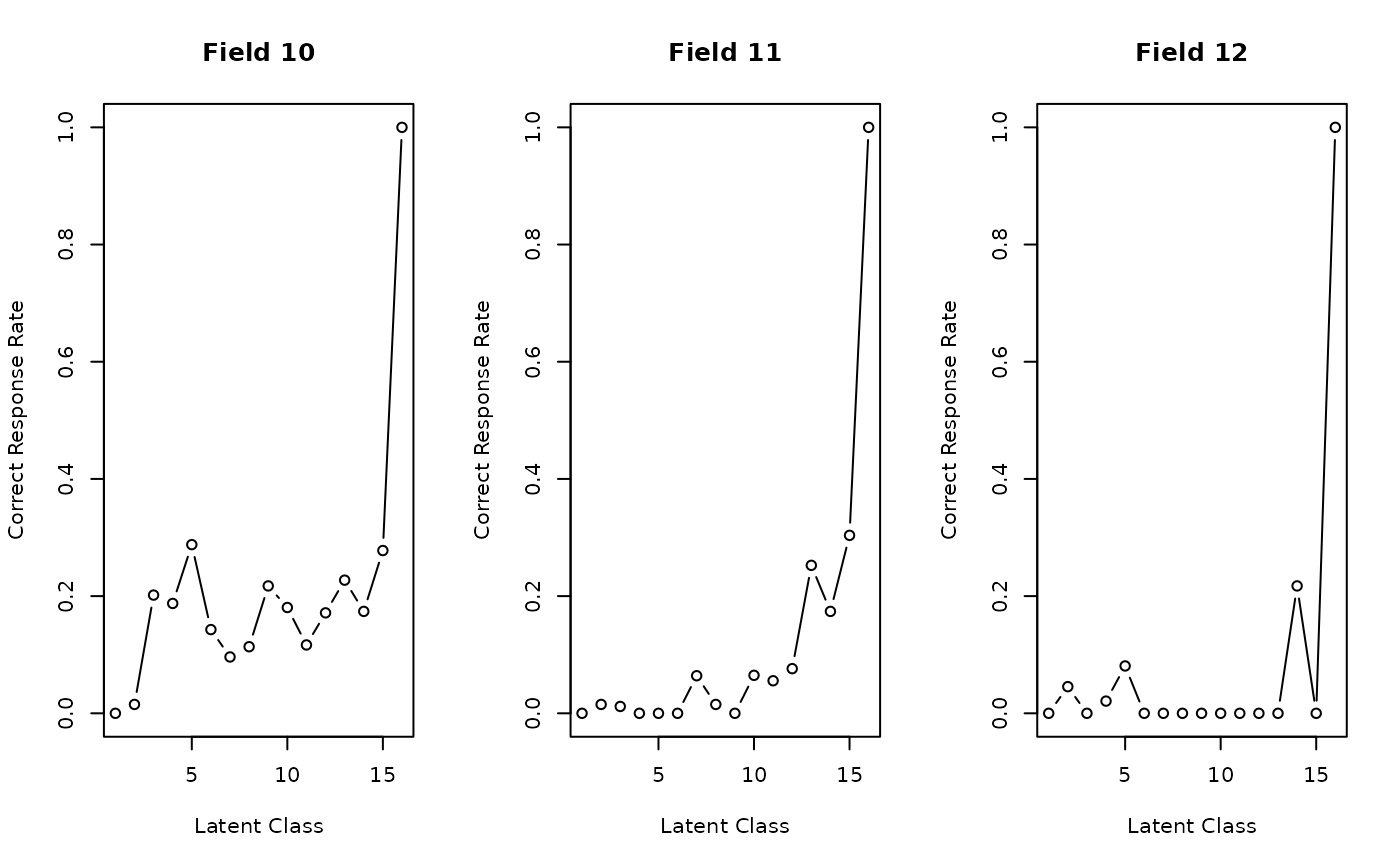
FRP: Field Reference Profile
FRPIndex: Index of FFP includes the item location parameters B and Beta, the slope parameters A and Alpha, and the monotonicity indices C and Gamma.
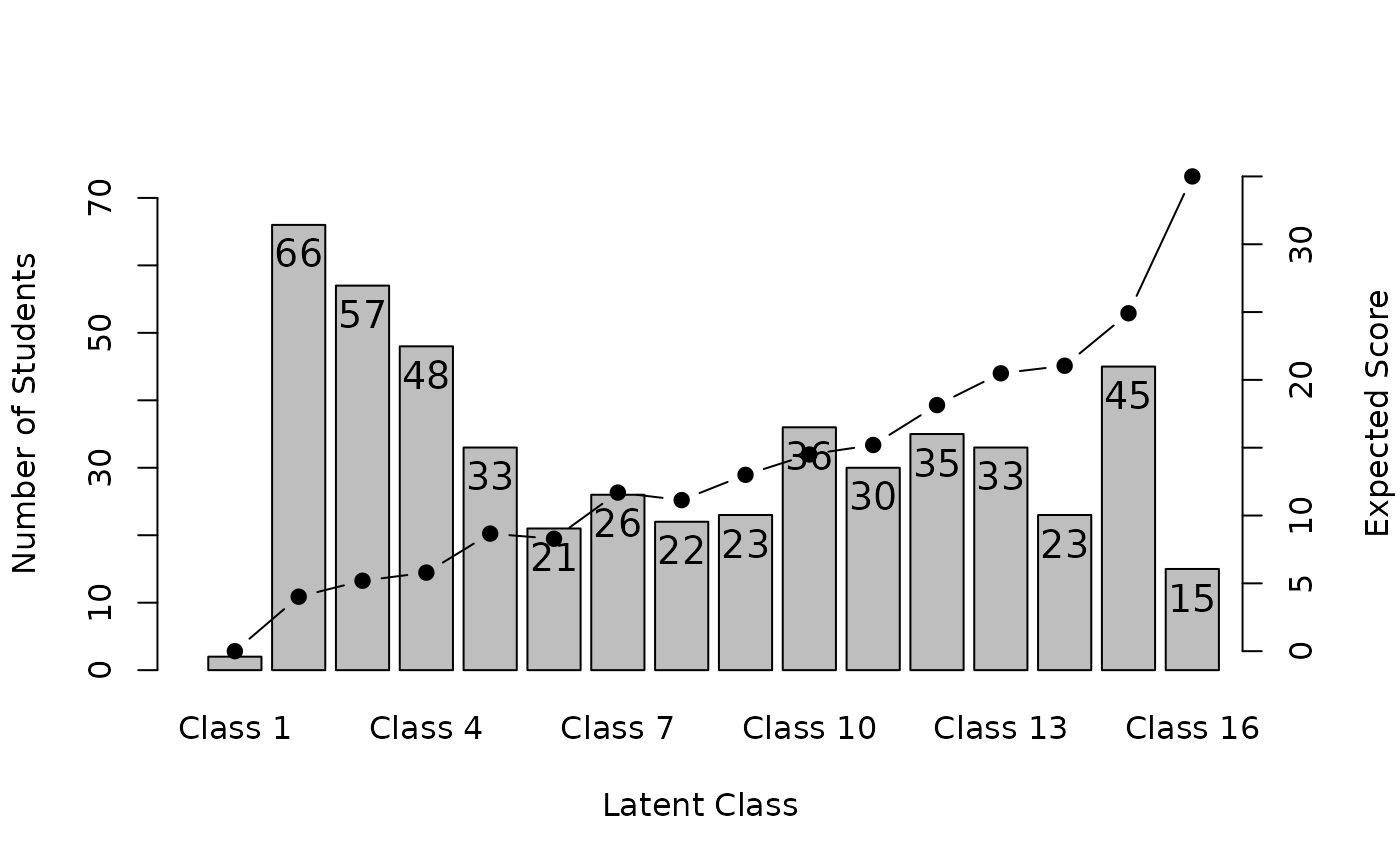
TRP: Test Reference Profile
FMP: Field Membership Profile
Students: Rank Membership Profile matrix.The s-th row vector of \(\hat{M}_R\), \(\hat{m}_R\), is the rank membership profile of Student s, namely the posterior probability distribution representing the student's belonging to the respective latent classes. It also includes the rank with the maximum estimated membership probability, as well as the rank-up odds and rank-down odds.
LRD: Latent Rank Distribution. see also plot.exametrika
LFD: Latent Field Distribution. see also plot.exametrika
RMD: Rank Membership Distribution.
TestFitIndices: Overall fit index for the test.See also TestFit

For nominal data, the returned list includes:

Q: Response matrix.
Z: Missing indicator matrix.
testlength: Number of items.
nobs: Sample size.
n_class: Optimal number of classes.
n_field: Optimal number of fields.
n_cycle: Number of EM algorithm iterations.
FRP: Field Reference Profile, a 3D array (nfld x ncls x maxQ).
LFD: Latent Field Distribution.
LCD: Latent Class Distribution.
FieldMembership: Field membership probability matrix.
ClassMembership: Class membership probability matrix.
FieldEstimated: Estimated field assignment for each item.
ClassEstimated: Estimated class assignment for each student.
Students: Rank Membership Profile matrix with estimated class.
TestFitIndices: Overall fit index for the test.
log_lik: Log-likelihood of the model.

For ordinal data, the returned list includes:

Q: Response matrix.
Z: Missing indicator matrix.
testlength: Number of items.
nobs: Sample size.
n_class: Optimal number of classes.
n_field: Optimal number of fields.
n_cycle: Number of EM algorithm iterations.
FRP: Field Reference Profile (BCRM), a 3D array (nfld x ncls x maxQ).
FRPIndex: Index of FRP includes the item location parameters B and Beta, the slope parameters A and Alpha, and the monotonicity indices C and Gamma.
TRP: Test Reference Profile.
BFRP: Bicluster Field Reference Profile (expected scores), a list with Weighted and Observed components.
LFD: Latent Field Distribution.
LCD: Latent Class Distribution.
FieldMembership: Field membership probability matrix.
ClassMembership: Class membership probability matrix.
FieldEstimated: Estimated field assignment for each item.
ClassEstimated: Estimated class assignment for each student.
Students: Rank Membership Profile matrix with estimated class.
TestFitIndices: Overall fit index for the test.
log_lik: Log-likelihood of the model.
SOACflg: Logical; TRUE if Strongly Ordinal Alignment Condition is satisfied.
WOACflg: Logical; TRUE if Weakly Ordinal Alignment Condition is satisfied.

Examples

# \donttest{
# Fit a Biclustering model with automatic structure learning using IRM
# gamma_c and gamma_f are concentration parameters for the Chinese Restaurant Process
result <- Biclustering_IRM(J35S515, gamma_c = 1, gamma_f = 1, verbose = TRUE)
#> iter 1: match=0 nfld=15 ncls=30
#> iter 2: match=0 nfld=12 ncls=27
#> iter 3: match=1 nfld=12 ncls=24
#> iter 4: match=2 nfld=12 ncls=23
#> iter 5: match=3 nfld=12 ncls=23
#> iter 6: match=0 nfld=12 ncls=23
#> iter 7: match=1 nfld=12 ncls=23
#> iter 8: match=2 nfld=12 ncls=23
#> iter 9: match=3 nfld=12 ncls=21
#> iter 10: match=4 nfld=12 ncls=21
#> iter 11: match=5 nfld=12 ncls=21
#> Adjusting classes: BIC=-99592.5 ncls=21 (min size < 20)
#> Adjusting classes: BIC=-99980.4 ncls=20 (min size < 20)
#> Adjusting classes: BIC=-99959.7 ncls=19 (min size < 20)
#> Adjusting classes: BIC=-99988.3 ncls=18 (min size < 20)
#> Adjusting classes: BIC=-100001.3 ncls=17 (min size < 20)

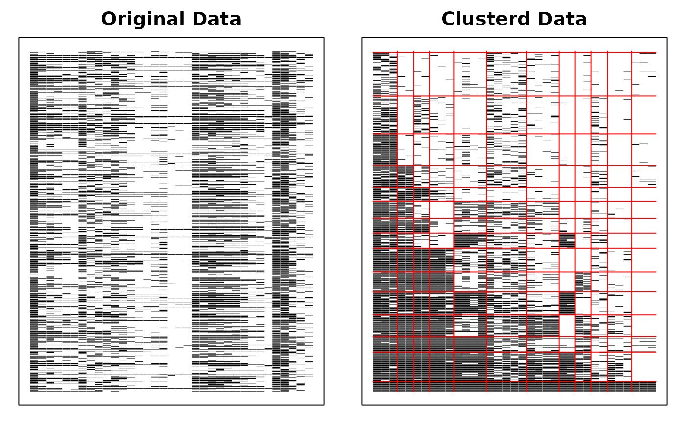
# Display the Bicluster Reference Matrix (BRM) as a heatmap
plot(result, type = "Array")


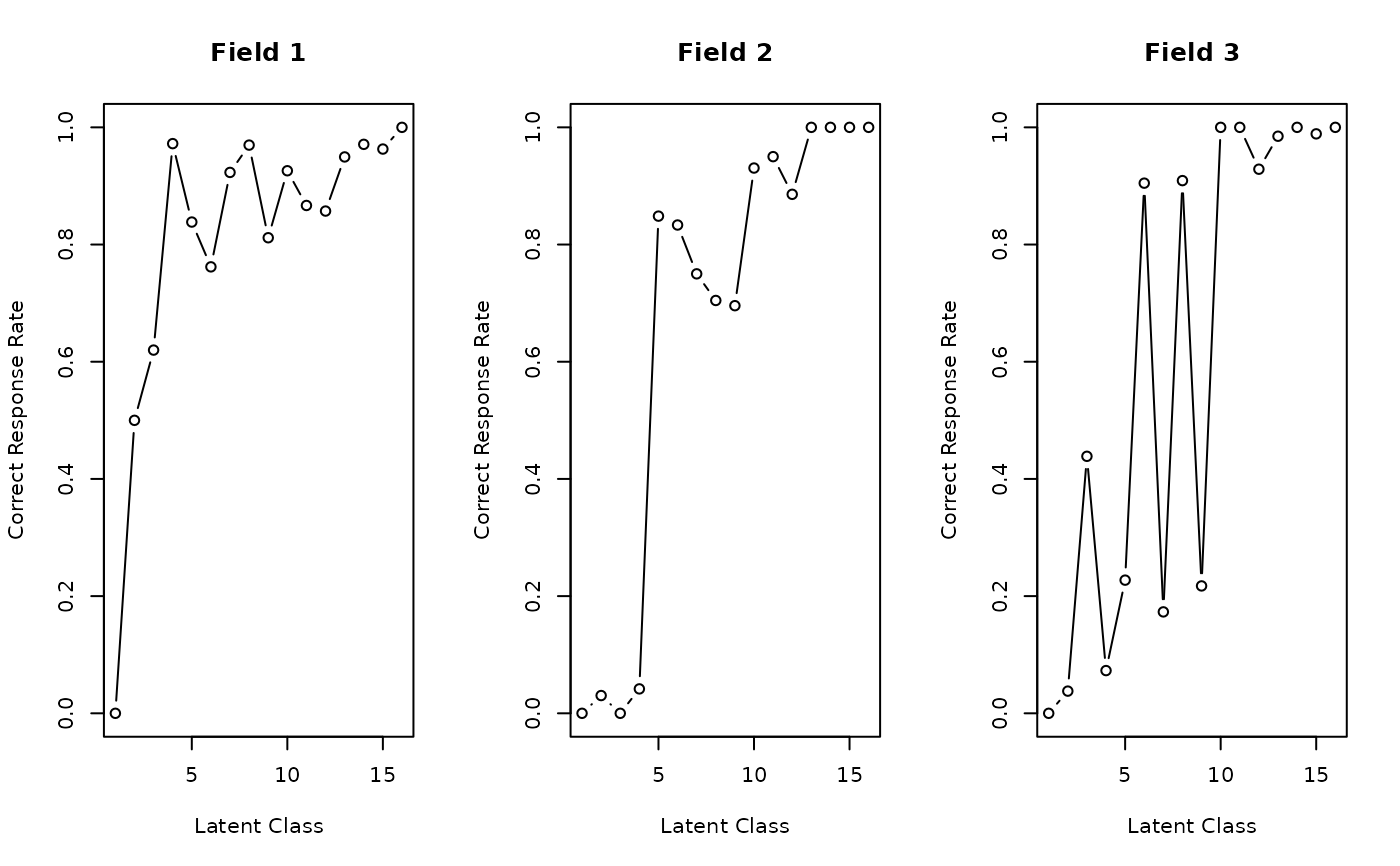
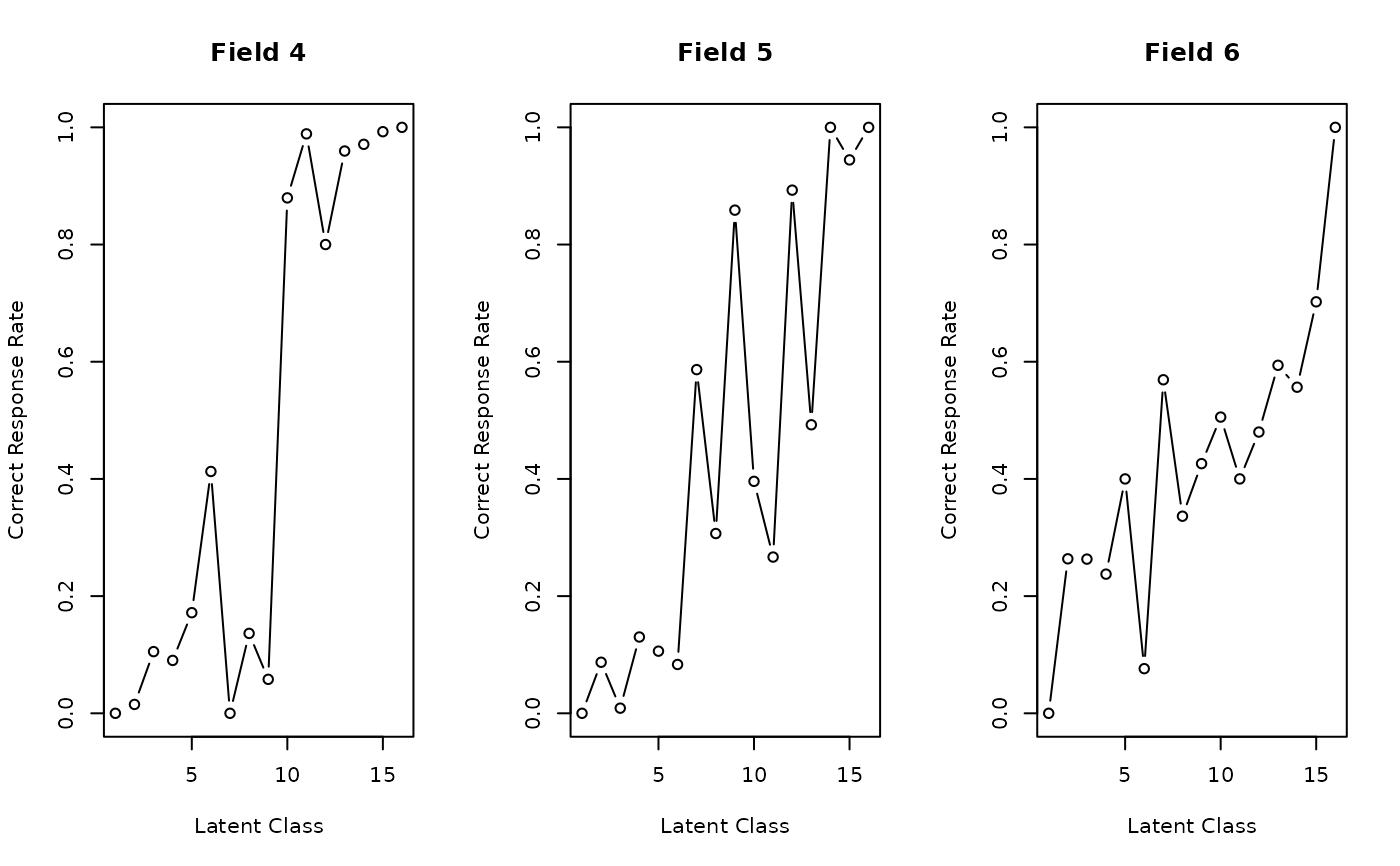
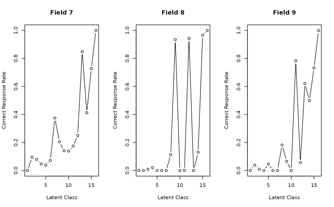
# Plot Field Reference Profiles (FRP) in a 3-column grid
plot(result, type = "FRP", nc = 3)




# }

# \donttest{
result <- Biclustering_IRM(J35S515, gamma_c = 1, gamma_f = 1, verbose = TRUE)
#> iter 1: match=0 nfld=15 ncls=30
#> iter 2: match=0 nfld=12 ncls=27
#> iter 3: match=1 nfld=12 ncls=24
#> iter 4: match=2 nfld=12 ncls=23
#> iter 5: match=3 nfld=12 ncls=23
#> iter 6: match=0 nfld=12 ncls=23
#> iter 7: match=1 nfld=12 ncls=23
#> iter 8: match=2 nfld=12 ncls=23
#> iter 9: match=3 nfld=12 ncls=21
#> iter 10: match=4 nfld=12 ncls=21
#> iter 11: match=5 nfld=12 ncls=21
#> Adjusting classes: BIC=-99592.5 ncls=21 (min size < 20)
#> Adjusting classes: BIC=-99980.4 ncls=20 (min size < 20)
#> Adjusting classes: BIC=-99959.7 ncls=19 (min size < 20)
#> Adjusting classes: BIC=-99988.3 ncls=18 (min size < 20)
#> Adjusting classes: BIC=-100001.3 ncls=17 (min size < 20)
plot(result, type = "Array")

# }
# \donttest{
# Fit a nominal Biclustering IRM model
result <- Biclustering_IRM(J20S600, gamma_c = 1, gamma_f = 1, verbose = TRUE)
#> iter 1: match=0 nfld=6 ncls=6
#> iter 2: match=0 nfld=4 ncls=6
#> iter 3: match=1 nfld=4 ncls=7
#> iter 4: match=2 nfld=4 ncls=7
#> iter 5: match=3 nfld=4 ncls=5
#> iter 6: match=4 nfld=4 ncls=6
#> iter 7: match=5 nfld=4 ncls=6
#> Adjusting classes: BIC=28686.8 ncls=6 (min size < 20)
plot(result, type = "Array")

# }
# \donttest{
# Fit an ordinal Biclustering IRM model
result <- Biclustering_IRM(J35S500, gamma_c = 1, gamma_f = 1, verbose = TRUE)
#> iter 1: match=0 nfld=13 ncls=46
#> iter 2: match=0 nfld=8 ncls=30
#> iter 3: match=0 nfld=6 ncls=18
#> iter 4: match=1 nfld=6 ncls=11
#> iter 5: match=0 nfld=5 ncls=10
#> iter 6: match=1 nfld=5 ncls=10
#> iter 7: match=2 nfld=5 ncls=9
#> iter 8: match=3 nfld=5 ncls=7
#> iter 9: match=4 nfld=5 ncls=6
#> iter 10: match=5 nfld=5 ncls=6
#> Weakly ordinal alignment condition was satisfied.
plot(result, type = "Array")

# }