Latent dependence Biclustering, which incorporates biclustering and a Bayesian network model.
Usage
LDB(
  U,
  na = NULL,
  Z = NULL,
  w = NULL,
  ncls = 2,
  method = "R",
  conf = NULL,
  g_list = NULL,
  adj_list = NULL,
  adj_file = NULL,
  verbose = FALSE,
  beta1 = 1,
  beta2 = 1
)
Arguments
- U
U is either a data class of exametrika, or raw data. When raw data is given, it is converted to the exametrika class with the dataFormat function.
- na
na argument specifies the numbers or characters to be treated as missing values.
- Z
Z is a missing indicator matrix of the type matrix or data.frame
- w
w is item weight vector
- ncls
number of latent class(rank). The default is 2.
- method
specify the model to analyze the data.Local dependence latent class model is set to "C", latent rank model is set "R". The default is "R".
- conf
For the confirmatory parameter, you can input either a vector with items and corresponding fields in sequence, or a field membership profile matrix. In the case of the former, the field membership profile matrix will be generated internally. When providing a membership profile matrix, it needs to be either matrix or data.frame. The number of fields(nfld) will be overwrite to the number of columns of this matrix.
- g_list
A list compiling graph-type objects for each rank/class.
- adj_list
A list compiling matrix-type adjacency matrices for each rank/class.
- adj_file
A file detailing the relationships of the graph for each rank/class, listed in the order of starting point, ending point, and rank(class).
- verbose
verbose output Flag. default is FALSE
- beta1
Beta distribution parameter 1 for prior density. Default is 1.
- beta2
Beta distribution parameter 2 for prior density. Default is 1.
Value
- nobs
Sample size. The number of rows in the dataset.
- testlength
Length of the test. The number of items included in the test.
- msg
A character string indicating the model type.
- Nclass
Optimal number of classes.
- Nfield
Optimal number of fields.
- crr
Correct Response Rate
- ItemLabel
Label of Items
- FieldLabel
Label of Fields
- adj_list
List of Adjacency matrix used in the model
- g_list
List of graph object used in the model
- IRP
List of Estimated Parameters. This object is three-dimensional PIRP array, where each dimension represents the number of rank,number of field, and Dmax. Dmax denotes the maximum number of correct response patterns for each field.
- LFD
Latent Field Distribution. see also plot.exametrika
- LRD
Latent Rank Distribution. see also plot.exametrika
- FRP
Marginal Field Reference Matrix
- FRPIndex
Index of FFP includes the item location parameters B and Beta, the slope parameters A and Alpha, and the monotonicity indices C and Gamma.
- CCRR_table
This table is a rearrangement of IRP into a data.frame format for output, consisting of combinations of rank ,field and PIRP.
- TRP
Test Reference Profile
- RMD
Rank Membership Distribution.
- FieldEstimated
Given vector which correspondence between items and the fields.
- ClassEstimated
An index indicating which class a student belongs to, estimated by confirmatory Ranklustering.
- Students
Rank Membership Profile matrix.The s-th row vector of \(\hat{M}_R\), \(\hat{m}_R\), is the rank membership profile of Student s, namely the posterior probability distribution representing the student's belonging to the respective latent classes. It also includes the rank with the maximum estimated membership probability, as well as the rank-up odds and rank-down odds.
- TestFitIndices
Overall fit index for the test.See also TestFit
Examples
# \donttest{
# Example: Latent Dirichlet Bayesian Network model
# Create field configuration vector based on field assignments
conf <- c(
1, 6, 6, 8, 9, 9, 4, 7, 7, 7, 5, 8, 9, 10, 10, 9, 9,
10, 10, 10, 2, 2, 3, 3, 5, 5, 6, 9, 9, 10, 1, 1, 7, 9, 10
)
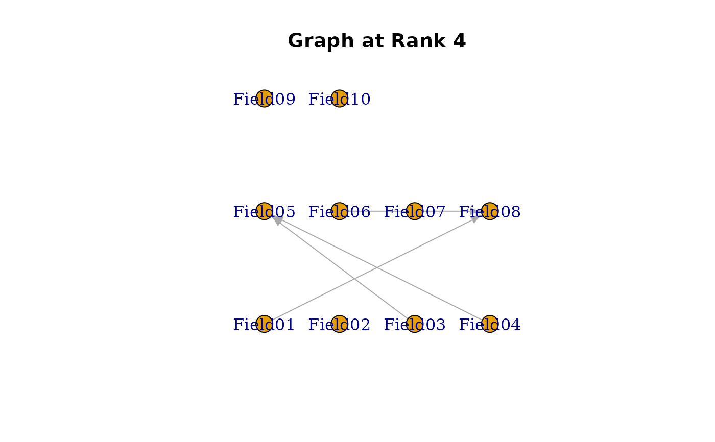
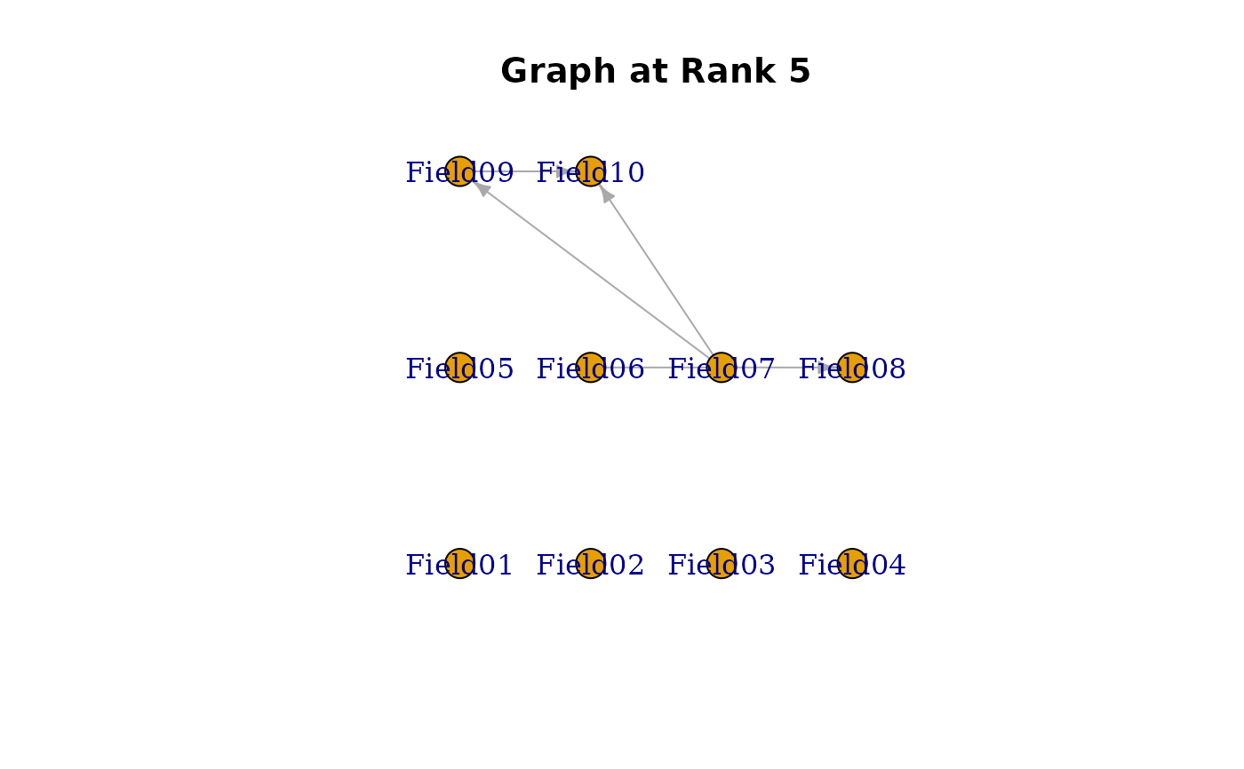
# Create edge data for the network structure between fields
edges_data <- data.frame(
"From Field (Parent) >>>" = c(
6, 4, 5, 1, 1, 4, # Class/Rank 2
3, 4, 6, 2, 4, 4, # Class/Rank 3
3, 6, 4, 1, # Class/Rank 4
7, 9, 6, 7 # Class/Rank 5
),
">>> To Field (Child)" = c(
8, 7, 8, 7, 2, 5, # Class/Rank 2
5, 8, 8, 4, 6, 7, # Class/Rank 3
5, 8, 5, 8, # Class/Rank 4
10, 10, 8, 9 # Class/Rank 5
),
"At Class/Rank (Locus)" = c(
2, 2, 2, 2, 2, 2, # Class/Rank 2
3, 3, 3, 3, 3, 3, # Class/Rank 3
4, 4, 4, 4, # Class/Rank 4
5, 5, 5, 5 # Class/Rank 5
)
)
# Save edge data to temporary CSV file
tmp_file <- tempfile(fileext = ".csv")
write.csv(edges_data, file = tmp_file, row.names = FALSE)
# Fit Latent Dirichlet Bayesian Network model
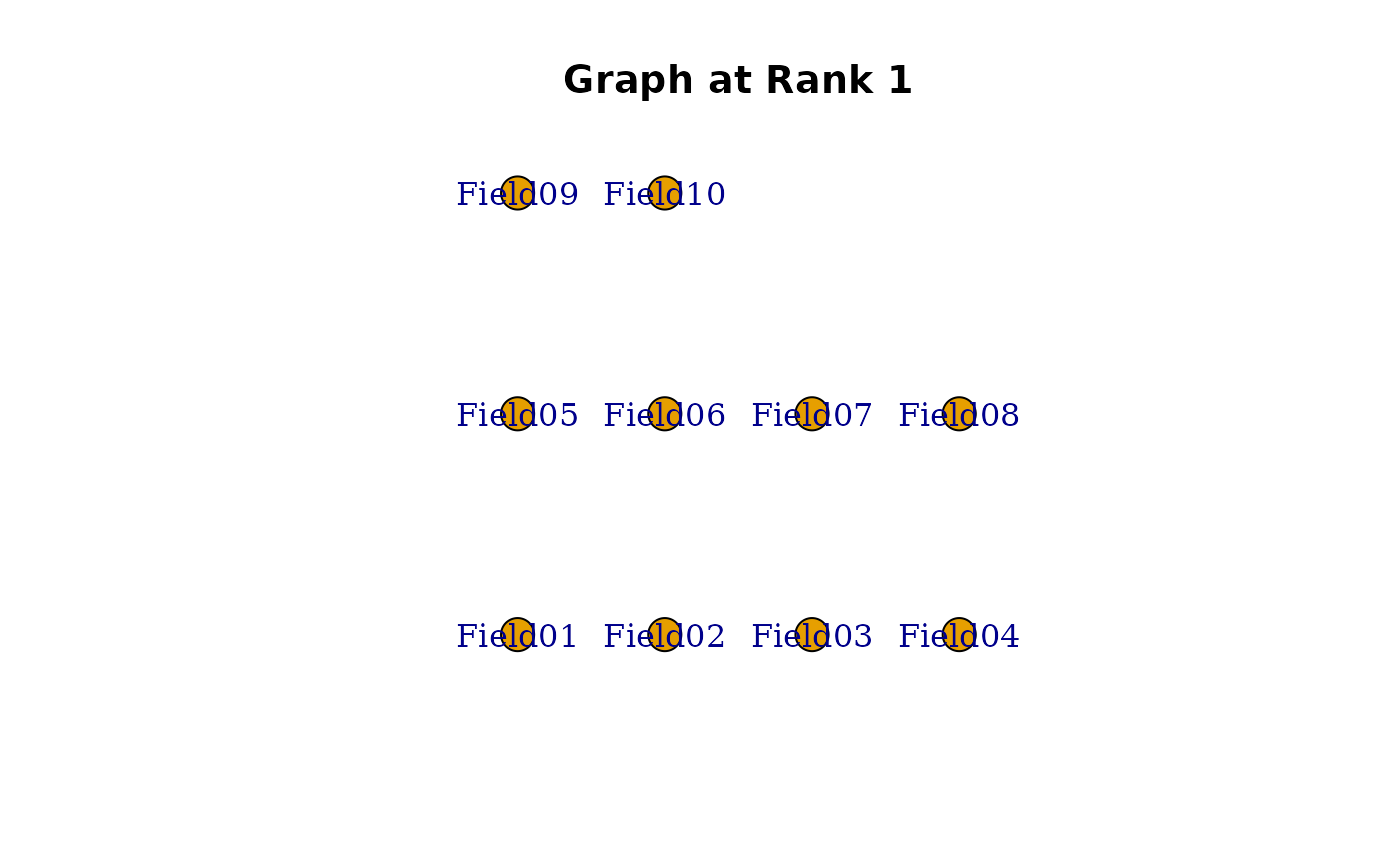
result.LDB <- LDB(
U = J35S515,
ncls = 5, # Number of latent classes
conf = conf, # Field configuration vector
adj_file = tmp_file # Path to the CSV file
)
# Clean up temporary file
unlink(tmp_file)
# Display model results
print(result.LDB)
#> Adjacency Matrix
#> [[1]]
#> Field01 Field02 Field03 Field04 Field05 Field06 Field07 Field08 Field09
#> Field01 0 0 0 0 0 0 0 0 0
#> Field02 0 0 0 0 0 0 0 0 0
#> Field03 0 0 0 0 0 0 0 0 0
#> Field04 0 0 0 0 0 0 0 0 0
#> Field05 0 0 0 0 0 0 0 0 0
#> Field06 0 0 0 0 0 0 0 0 0
#> Field07 0 0 0 0 0 0 0 0 0
#> Field08 0 0 0 0 0 0 0 0 0
#> Field09 0 0 0 0 0 0 0 0 0
#> Field10 0 0 0 0 0 0 0 0 0
#> Field10
#> Field01 0
#> Field02 0
#> Field03 0
#> Field04 0
#> Field05 0
#> Field06 0
#> Field07 0
#> Field08 0
#> Field09 0
#> Field10 0
#>
#> [[2]]
#> Field01 Field02 Field03 Field04 Field05 Field06 Field07 Field08 Field09
#> Field01 0 1 0 0 0 0 1 0 0
#> Field02 0 0 0 0 0 0 0 0 0
#> Field03 0 0 0 0 0 0 0 0 0
#> Field04 0 0 0 0 1 0 1 0 0
#> Field05 0 0 0 0 0 0 0 1 0
#> Field06 0 0 0 0 0 0 0 1 0
#> Field07 0 0 0 0 0 0 0 0 0
#> Field08 0 0 0 0 0 0 0 0 0
#> Field09 0 0 0 0 0 0 0 0 0
#> Field10 0 0 0 0 0 0 0 0 0
#> Field10
#> Field01 0
#> Field02 0
#> Field03 0
#> Field04 0
#> Field05 0
#> Field06 0
#> Field07 0
#> Field08 0
#> Field09 0
#> Field10 0
#>
#> [[3]]
#> Field01 Field02 Field03 Field04 Field05 Field06 Field07 Field08 Field09
#> Field01 0 0 0 0 0 0 0 0 0
#> Field02 0 0 0 1 0 0 0 0 0
#> Field03 0 0 0 0 1 0 0 0 0
#> Field04 0 0 0 0 0 1 1 1 0
#> Field05 0 0 0 0 0 0 0 0 0
#> Field06 0 0 0 0 0 0 0 1 0
#> Field07 0 0 0 0 0 0 0 0 0
#> Field08 0 0 0 0 0 0 0 0 0
#> Field09 0 0 0 0 0 0 0 0 0
#> Field10 0 0 0 0 0 0 0 0 0
#> Field10
#> Field01 0
#> Field02 0
#> Field03 0
#> Field04 0
#> Field05 0
#> Field06 0
#> Field07 0
#> Field08 0
#> Field09 0
#> Field10 0
#>
#> [[4]]
#> Field01 Field02 Field03 Field04 Field05 Field06 Field07 Field08 Field09
#> Field01 0 0 0 0 0 0 0 1 0
#> Field02 0 0 0 0 0 0 0 0 0
#> Field03 0 0 0 0 1 0 0 0 0
#> Field04 0 0 0 0 1 0 0 0 0
#> Field05 0 0 0 0 0 0 0 0 0
#> Field06 0 0 0 0 0 0 0 1 0
#> Field07 0 0 0 0 0 0 0 0 0
#> Field08 0 0 0 0 0 0 0 0 0
#> Field09 0 0 0 0 0 0 0 0 0
#> Field10 0 0 0 0 0 0 0 0 0
#> Field10
#> Field01 0
#> Field02 0
#> Field03 0
#> Field04 0
#> Field05 0
#> Field06 0
#> Field07 0
#> Field08 0
#> Field09 0
#> Field10 0
#>
#> [[5]]
#> Field01 Field02 Field03 Field04 Field05 Field06 Field07 Field08 Field09
#> Field01 0 0 0 0 0 0 0 0 0
#> Field02 0 0 0 0 0 0 0 0 0
#> Field03 0 0 0 0 0 0 0 0 0
#> Field04 0 0 0 0 0 0 0 0 0
#> Field05 0 0 0 0 0 0 0 0 0
#> Field06 0 0 0 0 0 0 0 1 0
#> Field07 0 0 0 0 0 0 0 0 1
#> Field08 0 0 0 0 0 0 0 0 0
#> Field09 0 0 0 0 0 0 0 0 0
#> Field10 0 0 0 0 0 0 0 0 0
#> Field10
#> Field01 0
#> Field02 0
#> Field03 0
#> Field04 0
#> Field05 0
#> Field06 0
#> Field07 1
#> Field08 0
#> Field09 1
#> Field10 0
#>


 #>
#> Parameter Learning
#> Rank 1
#> PIRP 0 PIRP 1 PIRP 2 PIRP 3 PIRP 4 PIRP 5 PIRP 6 PIRP 7 PIRP 8 PIRP 9
#> Field01 0.6538
#> Field02 0.0756
#> Field03 0.1835
#> Field04 0.3819
#> Field05 0.0500
#> Field06 0.0985
#> Field07 0.2176
#> Field08 0.0608
#> Field09 0.0563
#> Field10 0.0237
#> PIRP 10 PIRP 11 PIRP 12
#> Field01
#> Field02
#> Field03
#> Field04
#> Field05
#> Field06
#> Field07
#> Field08
#> Field09
#> Field10
#> Rank 2
#> PIRP 0 PIRP 1 PIRP 2 PIRP 3 PIRP 4 PIRP 5 PIRP 6 PIRP 7 PIRP 8 PIRP 9
#> Field01 0.8216
#> Field02 0.1463 0.3181 0.383 0.597
#> Field03 0.3320
#> Field04 0.4931
#> Field05 0.1596 0.2552
#> Field06 0.2541
#> Field07 0.1232 0.2926 0.217 0.306 0.376
#> Field08 0.0648 0.0887 0.236 0.443 0.196 0.285 0.624
#> Field09 0.1101
#> Field10 0.0359
#> PIRP 10 PIRP 11 PIRP 12
#> Field01
#> Field02
#> Field03
#> Field04
#> Field05
#> Field06
#> Field07
#> Field08
#> Field09
#> Field10
#> Rank 3
#> PIRP 0 PIRP 1 PIRP 2 PIRP 3 PIRP 4 PIRP 5 PIRP 6 PIRP 7 PIRP 8 PIRP 9
#> Field01 0.8923
#> Field02 0.8736
#> Field03 0.8030
#> Field04 0.4730 0.492 0.650
#> Field05 0.2732 0.319 0.714
#> Field06 0.4025 0.486
#> Field07 0.3162 0.408
#> Field08 0.1028 0.166 0.177 0.439 0.59
#> Field09 0.1799
#> Field10 0.0431
#> PIRP 10 PIRP 11 PIRP 12
#> Field01
#> Field02
#> Field03
#> Field04
#> Field05
#> Field06
#> Field07
#> Field08
#> Field09
#> Field10
#> Rank 4
#> PIRP 0 PIRP 1 PIRP 2 PIRP 3 PIRP 4 PIRP 5 PIRP 6 PIRP 7 PIRP 8
#> Field01 0.91975
#> Field02 0.97126
#> Field03 0.96955
#> Field04 0.70098
#> Field05 0.28691 0.476702 0.911 0.952
#> Field06 0.72620
#> Field07 0.48152
#> Field08 0.00353 0.000122 0.370 0.370 0.401 0.532 0.779
#> Field09 0.36220
#> Field10 0.08630
#> PIRP 9 PIRP 10 PIRP 11 PIRP 12
#> Field01
#> Field02
#> Field03
#> Field04
#> Field05
#> Field06
#> Field07
#> Field08
#> Field09
#> Field10
#> Rank 5
#> PIRP 0 PIRP 1 PIRP 2 PIRP 3 PIRP 4 PIRP 5 PIRP 6 PIRP 7 PIRP 8 PIRP 9
#> Field01 0.9627
#> Field02 0.9959
#> Field03 0.9947
#> Field04 0.8654
#> Field05 0.9939
#> Field06 0.9178
#> Field07 0.7334
#> Field08 0.5109 0.4442 0.5939 0.9174
#> Field09 0.4062 0.5193 0.6496 0.6786 0.851
#> Field10 0.0874 0.0278 0.0652 0.0429 0.110 0.117 0.118 0.163 0.217 0.275
#> PIRP 10 PIRP 11 PIRP 12
#> Field01
#> Field02
#> Field03
#> Field04
#> Field05
#> Field06
#> Field07
#> Field08
#> Field09
#> Field10 0.262 0.257 0.95
#>
#> Marginal Rankluster Reference Matrix
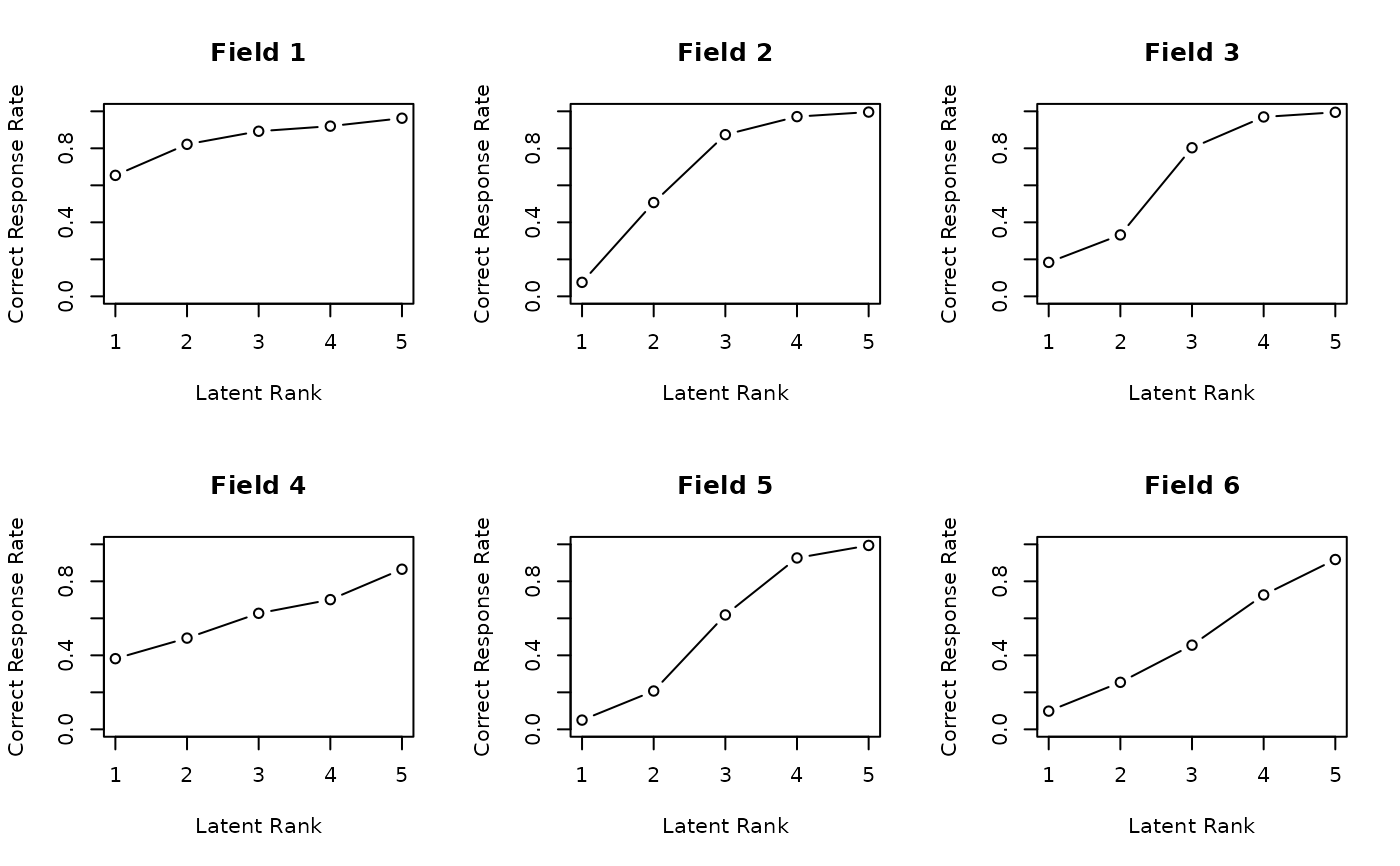
#> Rank 1 Rank 2 Rank 3 Rank 4 Rank 5
#> Field01 0.6538 0.8216 0.8923 0.9198 0.963
#> Field02 0.0756 0.5069 0.8736 0.9713 0.996
#> Field03 0.1835 0.3320 0.8030 0.9696 0.995
#> Field04 0.3819 0.4931 0.6271 0.7010 0.865
#> Field05 0.0500 0.2072 0.6182 0.9263 0.994
#> Field06 0.0985 0.2541 0.4550 0.7262 0.918
#> Field07 0.2176 0.3119 0.3738 0.4815 0.733
#> Field08 0.0608 0.1723 0.2718 0.5700 0.863
#> Field09 0.0563 0.1101 0.1799 0.3622 0.715
#> Field10 0.0237 0.0359 0.0431 0.0863 0.377
#>
#> IRP Indices
#> Alpha A Beta B Gamma C
#> Field01 1 0.168 1 0.654 0 0
#> Field02 1 0.431 2 0.507 0 0
#> Field03 2 0.471 2 0.332 0 0
#> Field04 4 0.164 2 0.493 0 0
#> Field05 2 0.411 3 0.618 0 0
#> Field06 3 0.271 3 0.455 0 0
#> Field07 4 0.252 4 0.482 0 0
#> Field08 3 0.298 4 0.570 0 0
#> Field09 4 0.353 4 0.362 0 0
#> Field10 4 0.291 5 0.377 0 0
#> Rank 1 Rank 2 Rank 3 Rank 4 Rank 5
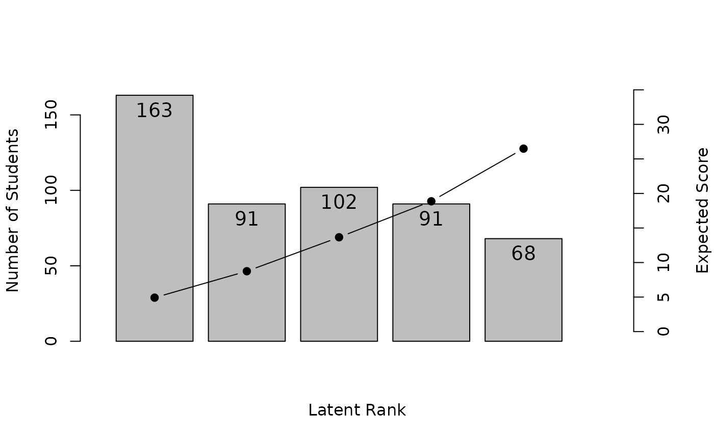
#> Test Reference Profile 4.915 8.744 13.657 18.867 26.488
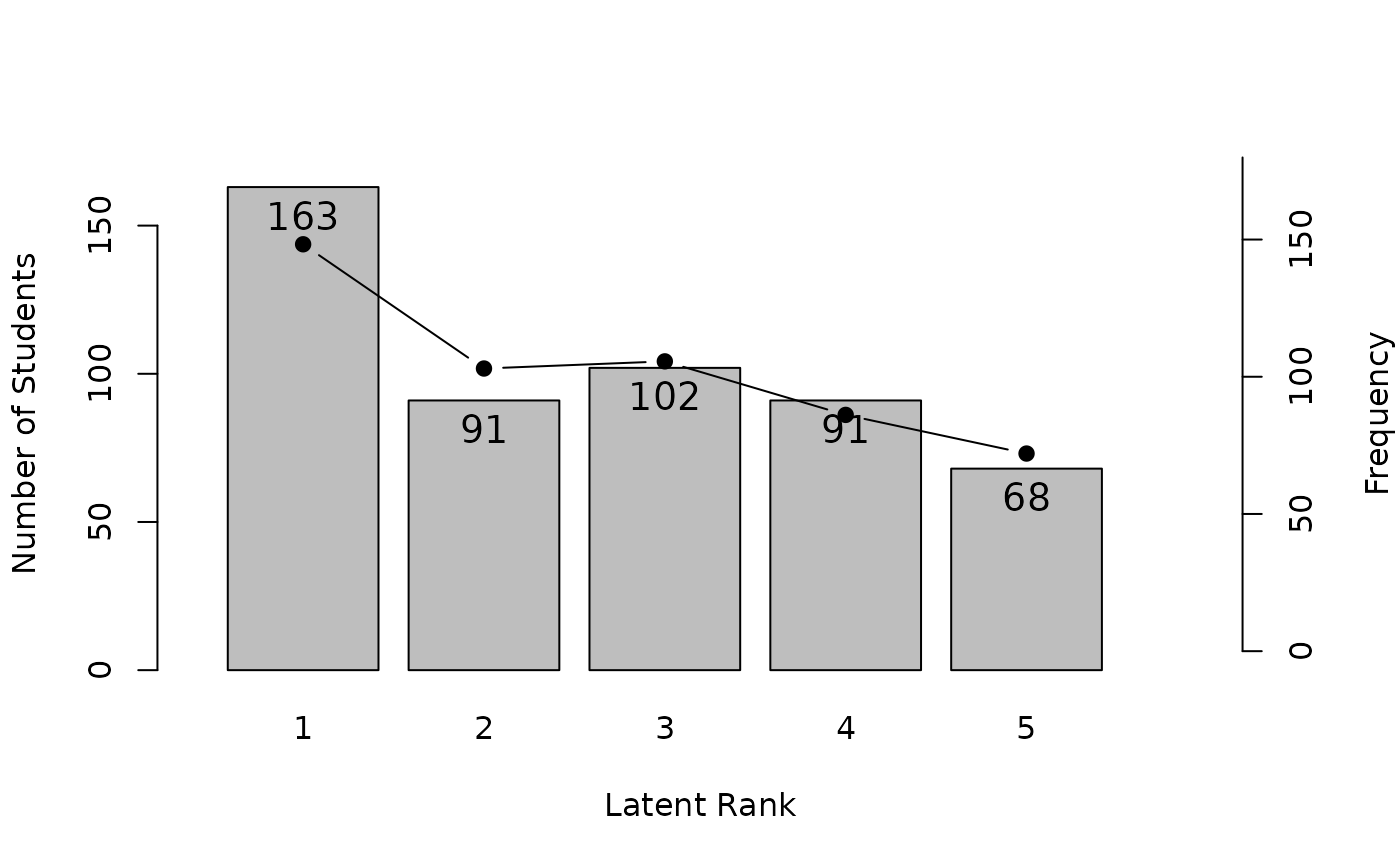
#> Latent Rank Ditribution 163.000 91.000 102.000 91.000 68.000
#> Rank Membership Dsitribution 148.275 103.002 105.606 86.100 72.017
#>
#> Latent Field Distribution
#> Field 1 Field 2 Field 3 Field 4 Field 5 Field 6 Field 7 Field 8
#> N of Items 3 2 2 1 3 3 4 2
#> Field 9 Field 10
#> N of Items 8 7
#>
#> Model Fit Indices
#> value
#> model_log_like -6804.899
#> bench_log_like -5891.314
#> null_log_like -9862.114
#> model_Chi_sq 1827.169
#> null_Chi_sq 7941.601
#> model_df 1088.000
#> null_df 1155.000
#> NFI 0.770
#> RFI 0.756
#> IFI 0.892
#> TLI 0.884
#> CFI 0.891
#> RMSEA 0.036
#> AIC -348.831
#> CAIC -6054.485
#> BIC -4966.485
#> Strongly ordinal alignment condition was satisfied.
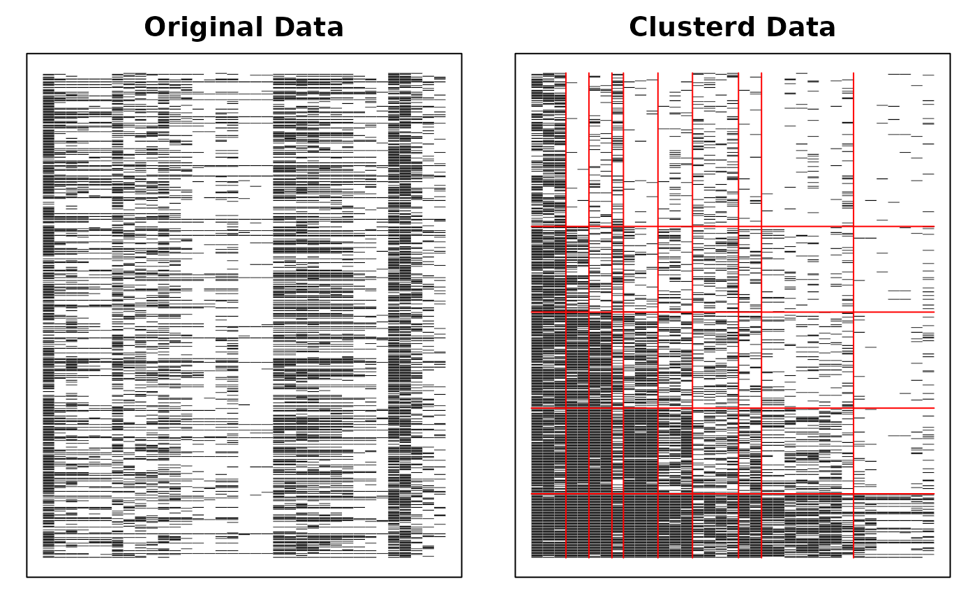
# Visualize different aspects of the model
plot(result.LDB, type = "Array") # Show bicluster structure
#>
#> Parameter Learning
#> Rank 1
#> PIRP 0 PIRP 1 PIRP 2 PIRP 3 PIRP 4 PIRP 5 PIRP 6 PIRP 7 PIRP 8 PIRP 9
#> Field01 0.6538
#> Field02 0.0756
#> Field03 0.1835
#> Field04 0.3819
#> Field05 0.0500
#> Field06 0.0985
#> Field07 0.2176
#> Field08 0.0608
#> Field09 0.0563
#> Field10 0.0237
#> PIRP 10 PIRP 11 PIRP 12
#> Field01
#> Field02
#> Field03
#> Field04
#> Field05
#> Field06
#> Field07
#> Field08
#> Field09
#> Field10
#> Rank 2
#> PIRP 0 PIRP 1 PIRP 2 PIRP 3 PIRP 4 PIRP 5 PIRP 6 PIRP 7 PIRP 8 PIRP 9
#> Field01 0.8216
#> Field02 0.1463 0.3181 0.383 0.597
#> Field03 0.3320
#> Field04 0.4931
#> Field05 0.1596 0.2552
#> Field06 0.2541
#> Field07 0.1232 0.2926 0.217 0.306 0.376
#> Field08 0.0648 0.0887 0.236 0.443 0.196 0.285 0.624
#> Field09 0.1101
#> Field10 0.0359
#> PIRP 10 PIRP 11 PIRP 12
#> Field01
#> Field02
#> Field03
#> Field04
#> Field05
#> Field06
#> Field07
#> Field08
#> Field09
#> Field10
#> Rank 3
#> PIRP 0 PIRP 1 PIRP 2 PIRP 3 PIRP 4 PIRP 5 PIRP 6 PIRP 7 PIRP 8 PIRP 9
#> Field01 0.8923
#> Field02 0.8736
#> Field03 0.8030
#> Field04 0.4730 0.492 0.650
#> Field05 0.2732 0.319 0.714
#> Field06 0.4025 0.486
#> Field07 0.3162 0.408
#> Field08 0.1028 0.166 0.177 0.439 0.59
#> Field09 0.1799
#> Field10 0.0431
#> PIRP 10 PIRP 11 PIRP 12
#> Field01
#> Field02
#> Field03
#> Field04
#> Field05
#> Field06
#> Field07
#> Field08
#> Field09
#> Field10
#> Rank 4
#> PIRP 0 PIRP 1 PIRP 2 PIRP 3 PIRP 4 PIRP 5 PIRP 6 PIRP 7 PIRP 8
#> Field01 0.91975
#> Field02 0.97126
#> Field03 0.96955
#> Field04 0.70098
#> Field05 0.28691 0.476702 0.911 0.952
#> Field06 0.72620
#> Field07 0.48152
#> Field08 0.00353 0.000122 0.370 0.370 0.401 0.532 0.779
#> Field09 0.36220
#> Field10 0.08630
#> PIRP 9 PIRP 10 PIRP 11 PIRP 12
#> Field01
#> Field02
#> Field03
#> Field04
#> Field05
#> Field06
#> Field07
#> Field08
#> Field09
#> Field10
#> Rank 5
#> PIRP 0 PIRP 1 PIRP 2 PIRP 3 PIRP 4 PIRP 5 PIRP 6 PIRP 7 PIRP 8 PIRP 9
#> Field01 0.9627
#> Field02 0.9959
#> Field03 0.9947
#> Field04 0.8654
#> Field05 0.9939
#> Field06 0.9178
#> Field07 0.7334
#> Field08 0.5109 0.4442 0.5939 0.9174
#> Field09 0.4062 0.5193 0.6496 0.6786 0.851
#> Field10 0.0874 0.0278 0.0652 0.0429 0.110 0.117 0.118 0.163 0.217 0.275
#> PIRP 10 PIRP 11 PIRP 12
#> Field01
#> Field02
#> Field03
#> Field04
#> Field05
#> Field06
#> Field07
#> Field08
#> Field09
#> Field10 0.262 0.257 0.95
#>
#> Marginal Rankluster Reference Matrix
#> Rank 1 Rank 2 Rank 3 Rank 4 Rank 5
#> Field01 0.6538 0.8216 0.8923 0.9198 0.963
#> Field02 0.0756 0.5069 0.8736 0.9713 0.996
#> Field03 0.1835 0.3320 0.8030 0.9696 0.995
#> Field04 0.3819 0.4931 0.6271 0.7010 0.865
#> Field05 0.0500 0.2072 0.6182 0.9263 0.994
#> Field06 0.0985 0.2541 0.4550 0.7262 0.918
#> Field07 0.2176 0.3119 0.3738 0.4815 0.733
#> Field08 0.0608 0.1723 0.2718 0.5700 0.863
#> Field09 0.0563 0.1101 0.1799 0.3622 0.715
#> Field10 0.0237 0.0359 0.0431 0.0863 0.377
#>
#> IRP Indices
#> Alpha A Beta B Gamma C
#> Field01 1 0.168 1 0.654 0 0
#> Field02 1 0.431 2 0.507 0 0
#> Field03 2 0.471 2 0.332 0 0
#> Field04 4 0.164 2 0.493 0 0
#> Field05 2 0.411 3 0.618 0 0
#> Field06 3 0.271 3 0.455 0 0
#> Field07 4 0.252 4 0.482 0 0
#> Field08 3 0.298 4 0.570 0 0
#> Field09 4 0.353 4 0.362 0 0
#> Field10 4 0.291 5 0.377 0 0
#> Rank 1 Rank 2 Rank 3 Rank 4 Rank 5
#> Test Reference Profile 4.915 8.744 13.657 18.867 26.488
#> Latent Rank Ditribution 163.000 91.000 102.000 91.000 68.000
#> Rank Membership Dsitribution 148.275 103.002 105.606 86.100 72.017
#>
#> Latent Field Distribution
#> Field 1 Field 2 Field 3 Field 4 Field 5 Field 6 Field 7 Field 8
#> N of Items 3 2 2 1 3 3 4 2
#> Field 9 Field 10
#> N of Items 8 7
#>
#> Model Fit Indices
#> value
#> model_log_like -6804.899
#> bench_log_like -5891.314
#> null_log_like -9862.114
#> model_Chi_sq 1827.169
#> null_Chi_sq 7941.601
#> model_df 1088.000
#> null_df 1155.000
#> NFI 0.770
#> RFI 0.756
#> IFI 0.892
#> TLI 0.884
#> CFI 0.891
#> RMSEA 0.036
#> AIC -348.831
#> CAIC -6054.485
#> BIC -4966.485
#> Strongly ordinal alignment condition was satisfied.
# Visualize different aspects of the model
plot(result.LDB, type = "Array") # Show bicluster structure
 plot(result.LDB, type = "TRP") # Test Response Profile
 plot(result.LDB, type = "LRD") # Latent Rank Distribution
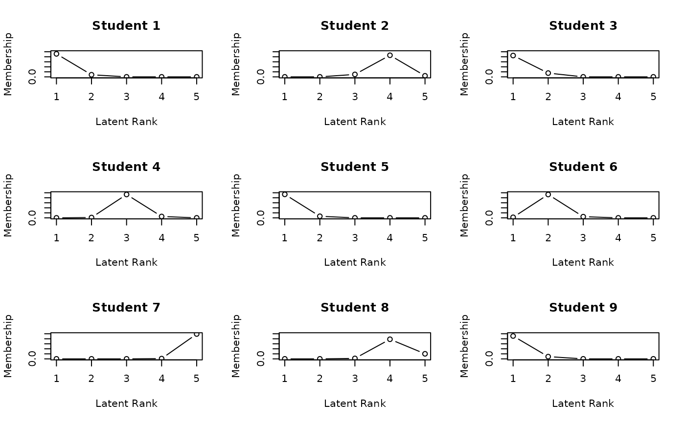
 plot(result.LDB,
type = "RMP", # Rank Membership Profiles
students = 1:9, nc = 3, nr = 3
)
plot(result.LDB,
type = "RMP", # Rank Membership Profiles
students = 1:9, nc = 3, nr = 3
)
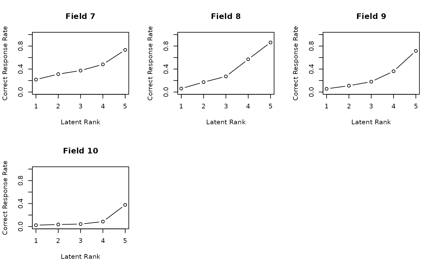
 plot(result.LDB,
type = "FRP", # Field Reference Profiles
nc = 3, nr = 2
)
plot(result.LDB,
type = "FRP", # Field Reference Profiles
nc = 3, nr = 2
)
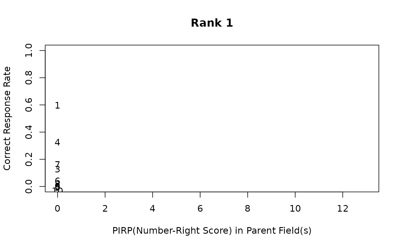
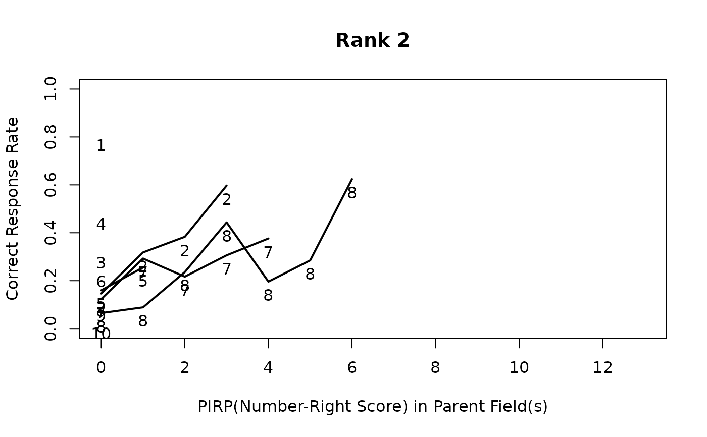
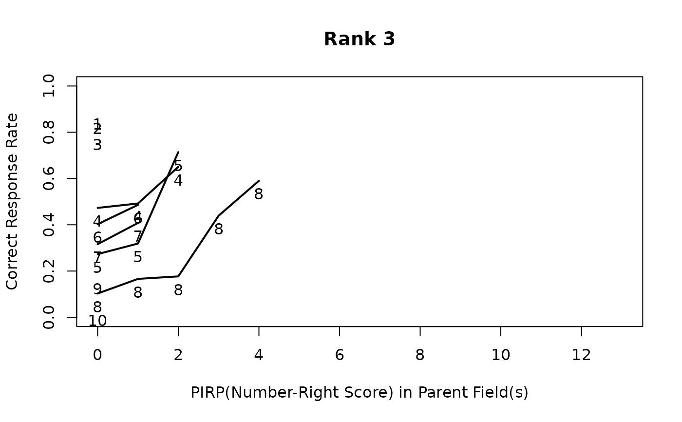
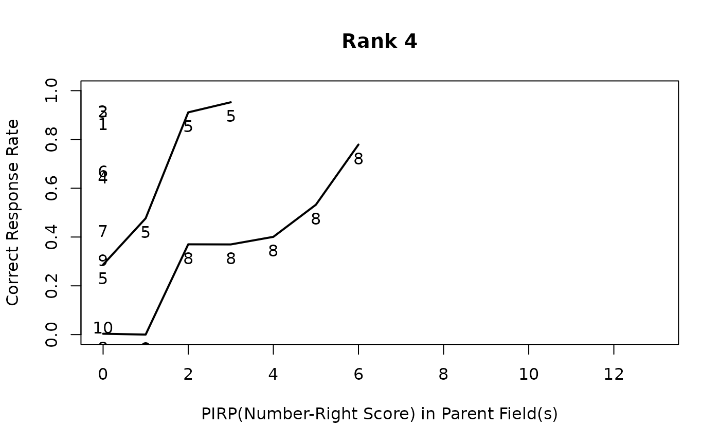
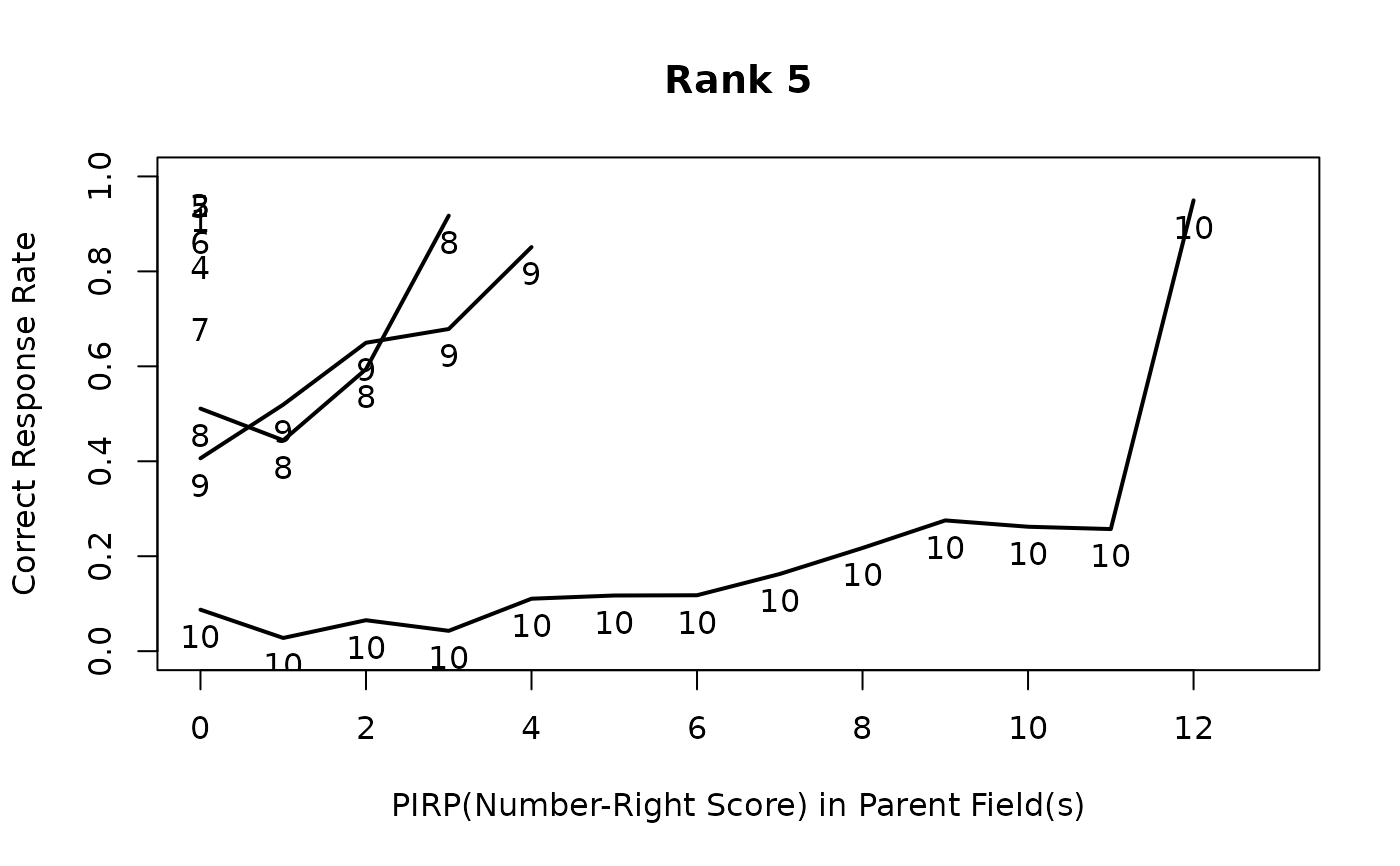
 # Field PIRP Profile showing correct answer counts for each rank and field
plot(result.LDB, type = "FieldPIRP")
# Field PIRP Profile showing correct answer counts for each rank and field
plot(result.LDB, type = "FieldPIRP")
 # }
# }