山大集中講義2019.03.09;Day 3-I

Day 3

始めるにあたって，プロジェクトフォルダを置くこと
下のコードを実行して，必要なパッケージを読み込んでおくこと

library(tidyverse)
# マカーの呪文
old = theme_set(theme_gray(base_family = "HiraKakuProN-W3"))
library(brms)

線形モデル5；階層線形モデル

こういうことがしたい。

read_csv('baseball2019.csv') %>% 
  # 野手のデータ
  dplyr::filter(position!="投手") %>% 
  # 年俸データを調整
  dplyr::mutate(salary = salary/1000) -> baseball_dat10

## Parsed with column specification:
## cols(
##   .default = col_double(),
##   Name = col_character(),
##   team = col_character(),
##   position = col_character(),
##   bloodType = col_character(),
##   throw.by = col_character(),
##   batting.by = col_character(),
##   birth.place = col_character(),
##   birth.day = col_date(format = ""),
##   背番号 = col_character()
## )

## See spec(...) for full column specifications.

baseball_dat10 %>% 
  # 描画
  ggplot(aes(x=安打,y=salary,color=team))+geom_point()+geom_smooth(method="lm",se=F)

## Warning: Removed 125 rows containing non-finite values (stat_smooth).

## Warning: Removed 125 rows containing missing values (geom_point).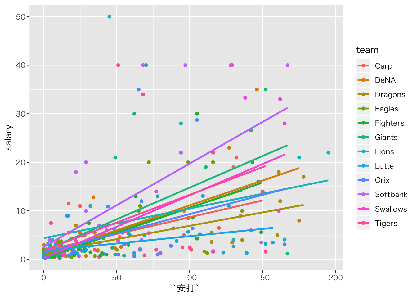

つまり，切片や傾きがチームごとによって違うようなモデルです。

ランダム切片モデル

切片だけが違うのはランダム切片モデルと言います。

# 年収のデータだから分布は対数正規分布
baseball_dat10 %>% 
  dplyr::select(salary,安打,team) %>% 
  na.omit() %>% 
  brm(salary~安打+(1|team),data=.,family="lognormal") -> result.hlm1

## Compiling the C++ model

## Start sampling

## 
## SAMPLING FOR MODEL 'aaf77108a5382a731933bf0a535b896a' NOW (CHAIN 1).
## Chain 1: 
## Chain 1: Gradient evaluation took 8.2e-05 seconds
## Chain 1: 1000 transitions using 10 leapfrog steps per transition would take 0.82 seconds.
## Chain 1: Adjust your expectations accordingly!
## Chain 1: 
## Chain 1: 
## Chain 1: Iteration:    1 / 2000 [  0%]  (Warmup)
## Chain 1: Iteration:  200 / 2000 [ 10%]  (Warmup)
## Chain 1: Iteration:  400 / 2000 [ 20%]  (Warmup)
## Chain 1: Iteration:  600 / 2000 [ 30%]  (Warmup)
## Chain 1: Iteration:  800 / 2000 [ 40%]  (Warmup)
## Chain 1: Iteration: 1000 / 2000 [ 50%]  (Warmup)
## Chain 1: Iteration: 1001 / 2000 [ 50%]  (Sampling)
## Chain 1: Iteration: 1200 / 2000 [ 60%]  (Sampling)
## Chain 1: Iteration: 1400 / 2000 [ 70%]  (Sampling)
## Chain 1: Iteration: 1600 / 2000 [ 80%]  (Sampling)
## Chain 1: Iteration: 1800 / 2000 [ 90%]  (Sampling)
## Chain 1: Iteration: 2000 / 2000 [100%]  (Sampling)
## Chain 1: 
## Chain 1:  Elapsed Time: 2.86567 seconds (Warm-up)
## Chain 1:                0.490072 seconds (Sampling)
## Chain 1:                3.35574 seconds (Total)
## Chain 1: 
## 
## SAMPLING FOR MODEL 'aaf77108a5382a731933bf0a535b896a' NOW (CHAIN 2).
## Chain 2: 
## Chain 2: Gradient evaluation took 4.9e-05 seconds
## Chain 2: 1000 transitions using 10 leapfrog steps per transition would take 0.49 seconds.
## Chain 2: Adjust your expectations accordingly!
## Chain 2: 
## Chain 2: 
## Chain 2: Iteration:    1 / 2000 [  0%]  (Warmup)
## Chain 2: Iteration:  200 / 2000 [ 10%]  (Warmup)
## Chain 2: Iteration:  400 / 2000 [ 20%]  (Warmup)
## Chain 2: Iteration:  600 / 2000 [ 30%]  (Warmup)
## Chain 2: Iteration:  800 / 2000 [ 40%]  (Warmup)
## Chain 2: Iteration: 1000 / 2000 [ 50%]  (Warmup)
## Chain 2: Iteration: 1001 / 2000 [ 50%]  (Sampling)
## Chain 2: Iteration: 1200 / 2000 [ 60%]  (Sampling)
## Chain 2: Iteration: 1400 / 2000 [ 70%]  (Sampling)
## Chain 2: Iteration: 1600 / 2000 [ 80%]  (Sampling)
## Chain 2: Iteration: 1800 / 2000 [ 90%]  (Sampling)
## Chain 2: Iteration: 2000 / 2000 [100%]  (Sampling)
## Chain 2: 
## Chain 2:  Elapsed Time: 2.55437 seconds (Warm-up)
## Chain 2:                0.524891 seconds (Sampling)
## Chain 2:                3.07926 seconds (Total)
## Chain 2: 
## 
## SAMPLING FOR MODEL 'aaf77108a5382a731933bf0a535b896a' NOW (CHAIN 3).
## Chain 3: 
## Chain 3: Gradient evaluation took 6.1e-05 seconds
## Chain 3: 1000 transitions using 10 leapfrog steps per transition would take 0.61 seconds.
## Chain 3: Adjust your expectations accordingly!
## Chain 3: 
## Chain 3: 
## Chain 3: Iteration:    1 / 2000 [  0%]  (Warmup)
## Chain 3: Iteration:  200 / 2000 [ 10%]  (Warmup)
## Chain 3: Iteration:  400 / 2000 [ 20%]  (Warmup)
## Chain 3: Iteration:  600 / 2000 [ 30%]  (Warmup)
## Chain 3: Iteration:  800 / 2000 [ 40%]  (Warmup)
## Chain 3: Iteration: 1000 / 2000 [ 50%]  (Warmup)
## Chain 3: Iteration: 1001 / 2000 [ 50%]  (Sampling)
## Chain 3: Iteration: 1200 / 2000 [ 60%]  (Sampling)
## Chain 3: Iteration: 1400 / 2000 [ 70%]  (Sampling)
## Chain 3: Iteration: 1600 / 2000 [ 80%]  (Sampling)
## Chain 3: Iteration: 1800 / 2000 [ 90%]  (Sampling)
## Chain 3: Iteration: 2000 / 2000 [100%]  (Sampling)
## Chain 3: 
## Chain 3:  Elapsed Time: 2.73431 seconds (Warm-up)
## Chain 3:                0.494847 seconds (Sampling)
## Chain 3:                3.22916 seconds (Total)
## Chain 3: 
## 
## SAMPLING FOR MODEL 'aaf77108a5382a731933bf0a535b896a' NOW (CHAIN 4).
## Chain 4: 
## Chain 4: Gradient evaluation took 6.3e-05 seconds
## Chain 4: 1000 transitions using 10 leapfrog steps per transition would take 0.63 seconds.
## Chain 4: Adjust your expectations accordingly!
## Chain 4: 
## Chain 4: 
## Chain 4: Iteration:    1 / 2000 [  0%]  (Warmup)
## Chain 4: Iteration:  200 / 2000 [ 10%]  (Warmup)
## Chain 4: Iteration:  400 / 2000 [ 20%]  (Warmup)
## Chain 4: Iteration:  600 / 2000 [ 30%]  (Warmup)
## Chain 4: Iteration:  800 / 2000 [ 40%]  (Warmup)
## Chain 4: Iteration: 1000 / 2000 [ 50%]  (Warmup)
## Chain 4: Iteration: 1001 / 2000 [ 50%]  (Sampling)
## Chain 4: Iteration: 1200 / 2000 [ 60%]  (Sampling)
## Chain 4: Iteration: 1400 / 2000 [ 70%]  (Sampling)
## Chain 4: Iteration: 1600 / 2000 [ 80%]  (Sampling)
## Chain 4: Iteration: 1800 / 2000 [ 90%]  (Sampling)
## Chain 4: Iteration: 2000 / 2000 [100%]  (Sampling)
## Chain 4: 
## Chain 4:  Elapsed Time: 2.70024 seconds (Warm-up)
## Chain 4:                0.486239 seconds (Sampling)
## Chain 4:                3.18648 seconds (Total)
## Chain 4:

result.hlm1

##  Family: lognormal 
##   Links: mu = identity; sigma = identity 
## Formula: salary ~ 安打 + (1 | team) 
##    Data: . (Number of observations: 322) 
## Samples: 4 chains, each with iter = 2000; warmup = 1000; thin = 1;
##          total post-warmup samples = 4000
## 
## Group-Level Effects: 
## ~team (Number of levels: 12) 
##               Estimate Est.Error l-95% CI u-95% CI Eff.Sample Rhat
## sd(Intercept)     0.09      0.07     0.00     0.25       2059 1.00
## 
## Population-Level Effects: 
##           Estimate Est.Error l-95% CI u-95% CI Eff.Sample Rhat
## Intercept     0.24      0.08     0.09     0.39       3642 1.00
## 安打          0.02      0.00     0.01     0.02       4239 1.00
## 
## Family Specific Parameters: 
##       Estimate Est.Error l-95% CI u-95% CI Eff.Sample Rhat
## sigma     0.94      0.04     0.87     1.02       5729 1.00
## 
## Samples were drawn using sampling(NUTS). For each parameter, Eff.Sample 
## is a crude measure of effective sample size, and Rhat is the potential 
## scale reduction factor on split chains (at convergence, Rhat = 1).

plot(result.hlm1)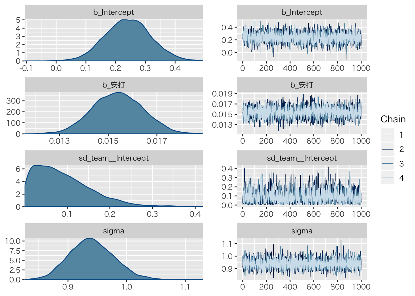

pp_check(result.hlm1)

## Using 10 posterior samples for ppc type 'dens_overlay' by default.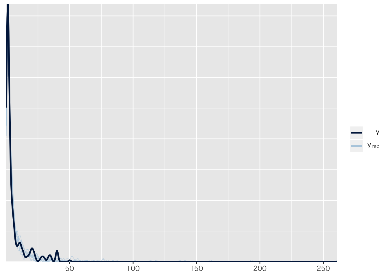

baseball_dat10 %>% 
  dplyr::select(salary,安打,team) %>% 
  na.omit() %>% 
  # 予測値をデータに追加
  cbind(fitted(result.hlm1)) %>% 
  ggplot(aes(安打, Estimate, color = team)) +
  geom_smooth(method = "lm", se = FALSE) +
  geom_point(aes(y = salary))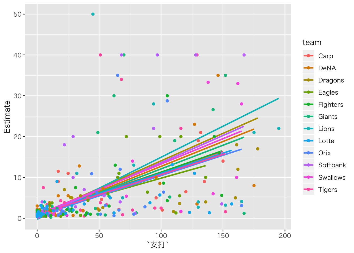

ランダム傾き・ランダム切片モデル

傾きもランダムにします。

# 年収のデータだから分布は対数正規分布
baseball_dat10 %>% 
  dplyr::select(salary,安打,team) %>% 
  na.omit() %>% 
  brm(salary~安打+(1+安打|team),data=.,family="lognormal") -> result.hlm2

## Compiling the C++ model

## Start sampling

## 
## SAMPLING FOR MODEL '3de93dbea09e0701426b1dcfaf30bf52' NOW (CHAIN 1).
## Chain 1: 
## Chain 1: Gradient evaluation took 0.000176 seconds
## Chain 1: 1000 transitions using 10 leapfrog steps per transition would take 1.76 seconds.
## Chain 1: Adjust your expectations accordingly!
## Chain 1: 
## Chain 1: 
## Chain 1: Iteration:    1 / 2000 [  0%]  (Warmup)
## Chain 1: Iteration:  200 / 2000 [ 10%]  (Warmup)
## Chain 1: Iteration:  400 / 2000 [ 20%]  (Warmup)
## Chain 1: Iteration:  600 / 2000 [ 30%]  (Warmup)
## Chain 1: Iteration:  800 / 2000 [ 40%]  (Warmup)
## Chain 1: Iteration: 1000 / 2000 [ 50%]  (Warmup)
## Chain 1: Iteration: 1001 / 2000 [ 50%]  (Sampling)
## Chain 1: Iteration: 1200 / 2000 [ 60%]  (Sampling)
## Chain 1: Iteration: 1400 / 2000 [ 70%]  (Sampling)
## Chain 1: Iteration: 1600 / 2000 [ 80%]  (Sampling)
## Chain 1: Iteration: 1800 / 2000 [ 90%]  (Sampling)
## Chain 1: Iteration: 2000 / 2000 [100%]  (Sampling)
## Chain 1: 
## Chain 1:  Elapsed Time: 4.39286 seconds (Warm-up)
## Chain 1:                0.760126 seconds (Sampling)
## Chain 1:                5.15298 seconds (Total)
## Chain 1: 
## 
## SAMPLING FOR MODEL '3de93dbea09e0701426b1dcfaf30bf52' NOW (CHAIN 2).
## Chain 2: 
## Chain 2: Gradient evaluation took 6.4e-05 seconds
## Chain 2: 1000 transitions using 10 leapfrog steps per transition would take 0.64 seconds.
## Chain 2: Adjust your expectations accordingly!
## Chain 2: 
## Chain 2: 
## Chain 2: Iteration:    1 / 2000 [  0%]  (Warmup)
## Chain 2: Iteration:  200 / 2000 [ 10%]  (Warmup)
## Chain 2: Iteration:  400 / 2000 [ 20%]  (Warmup)
## Chain 2: Iteration:  600 / 2000 [ 30%]  (Warmup)
## Chain 2: Iteration:  800 / 2000 [ 40%]  (Warmup)
## Chain 2: Iteration: 1000 / 2000 [ 50%]  (Warmup)
## Chain 2: Iteration: 1001 / 2000 [ 50%]  (Sampling)
## Chain 2: Iteration: 1200 / 2000 [ 60%]  (Sampling)
## Chain 2: Iteration: 1400 / 2000 [ 70%]  (Sampling)
## Chain 2: Iteration: 1600 / 2000 [ 80%]  (Sampling)
## Chain 2: Iteration: 1800 / 2000 [ 90%]  (Sampling)
## Chain 2: Iteration: 2000 / 2000 [100%]  (Sampling)
## Chain 2: 
## Chain 2:  Elapsed Time: 4.45157 seconds (Warm-up)
## Chain 2:                1.31639 seconds (Sampling)
## Chain 2:                5.76797 seconds (Total)
## Chain 2: 
## 
## SAMPLING FOR MODEL '3de93dbea09e0701426b1dcfaf30bf52' NOW (CHAIN 3).
## Chain 3: 
## Chain 3: Gradient evaluation took 7.7e-05 seconds
## Chain 3: 1000 transitions using 10 leapfrog steps per transition would take 0.77 seconds.
## Chain 3: Adjust your expectations accordingly!
## Chain 3: 
## Chain 3: 
## Chain 3: Iteration:    1 / 2000 [  0%]  (Warmup)
## Chain 3: Iteration:  200 / 2000 [ 10%]  (Warmup)
## Chain 3: Iteration:  400 / 2000 [ 20%]  (Warmup)
## Chain 3: Iteration:  600 / 2000 [ 30%]  (Warmup)
## Chain 3: Iteration:  800 / 2000 [ 40%]  (Warmup)
## Chain 3: Iteration: 1000 / 2000 [ 50%]  (Warmup)
## Chain 3: Iteration: 1001 / 2000 [ 50%]  (Sampling)
## Chain 3: Iteration: 1200 / 2000 [ 60%]  (Sampling)
## Chain 3: Iteration: 1400 / 2000 [ 70%]  (Sampling)
## Chain 3: Iteration: 1600 / 2000 [ 80%]  (Sampling)
## Chain 3: Iteration: 1800 / 2000 [ 90%]  (Sampling)
## Chain 3: Iteration: 2000 / 2000 [100%]  (Sampling)
## Chain 3: 
## Chain 3:  Elapsed Time: 4.12631 seconds (Warm-up)
## Chain 3:                0.771337 seconds (Sampling)
## Chain 3:                4.89765 seconds (Total)
## Chain 3: 
## 
## SAMPLING FOR MODEL '3de93dbea09e0701426b1dcfaf30bf52' NOW (CHAIN 4).
## Chain 4: 
## Chain 4: Gradient evaluation took 7.6e-05 seconds
## Chain 4: 1000 transitions using 10 leapfrog steps per transition would take 0.76 seconds.
## Chain 4: Adjust your expectations accordingly!
## Chain 4: 
## Chain 4: 
## Chain 4: Iteration:    1 / 2000 [  0%]  (Warmup)
## Chain 4: Iteration:  200 / 2000 [ 10%]  (Warmup)
## Chain 4: Iteration:  400 / 2000 [ 20%]  (Warmup)
## Chain 4: Iteration:  600 / 2000 [ 30%]  (Warmup)
## Chain 4: Iteration:  800 / 2000 [ 40%]  (Warmup)
## Chain 4: Iteration: 1000 / 2000 [ 50%]  (Warmup)
## Chain 4: Iteration: 1001 / 2000 [ 50%]  (Sampling)
## Chain 4: Iteration: 1200 / 2000 [ 60%]  (Sampling)
## Chain 4: Iteration: 1400 / 2000 [ 70%]  (Sampling)
## Chain 4: Iteration: 1600 / 2000 [ 80%]  (Sampling)
## Chain 4: Iteration: 1800 / 2000 [ 90%]  (Sampling)
## Chain 4: Iteration: 2000 / 2000 [100%]  (Sampling)
## Chain 4: 
## Chain 4:  Elapsed Time: 4.26654 seconds (Warm-up)
## Chain 4:                0.923678 seconds (Sampling)
## Chain 4:                5.19022 seconds (Total)
## Chain 4:

## Warning: There were 1 divergent transitions after warmup. Increasing adapt_delta above 0.8 may help. See
## http://mc-stan.org/misc/warnings.html#divergent-transitions-after-warmup

## Warning: Examine the pairs() plot to diagnose sampling problems

result.hlm2

## Warning: There were 1 divergent transitions after warmup. Increasing adapt_delta above 0.8 may help.
## See http://mc-stan.org/misc/warnings.html#divergent-transitions-after-warmup

##  Family: lognormal 
##   Links: mu = identity; sigma = identity 
## Formula: salary ~ 安打 + (1 + 安打 | team) 
##    Data: . (Number of observations: 322) 
## Samples: 4 chains, each with iter = 2000; warmup = 1000; thin = 1;
##          total post-warmup samples = 4000
## 
## Group-Level Effects: 
## ~team (Number of levels: 12) 
##                     Estimate Est.Error l-95% CI u-95% CI Eff.Sample Rhat
## sd(Intercept)           0.09      0.07     0.00     0.28       2378 1.00
## sd(安打)                0.00      0.00     0.00     0.00       1489 1.00
## cor(Intercept,安打)    -0.16      0.58    -0.97     0.92       1324 1.00
## 
## Population-Level Effects: 
##           Estimate Est.Error l-95% CI u-95% CI Eff.Sample Rhat
## Intercept     0.24      0.08     0.08     0.39       4184 1.00
## 安打          0.02      0.00     0.01     0.02       3410 1.00
## 
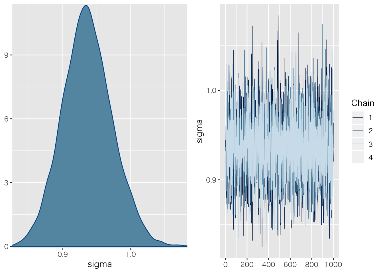
## Family Specific Parameters: 
##       Estimate Est.Error l-95% CI u-95% CI Eff.Sample Rhat
## sigma     0.94      0.04     0.87     1.01       4608 1.00
## 
## Samples were drawn using sampling(NUTS). For each parameter, Eff.Sample 
## is a crude measure of effective sample size, and Rhat is the potential 
## scale reduction factor on split chains (at convergence, Rhat = 1).

plot(result.hlm2)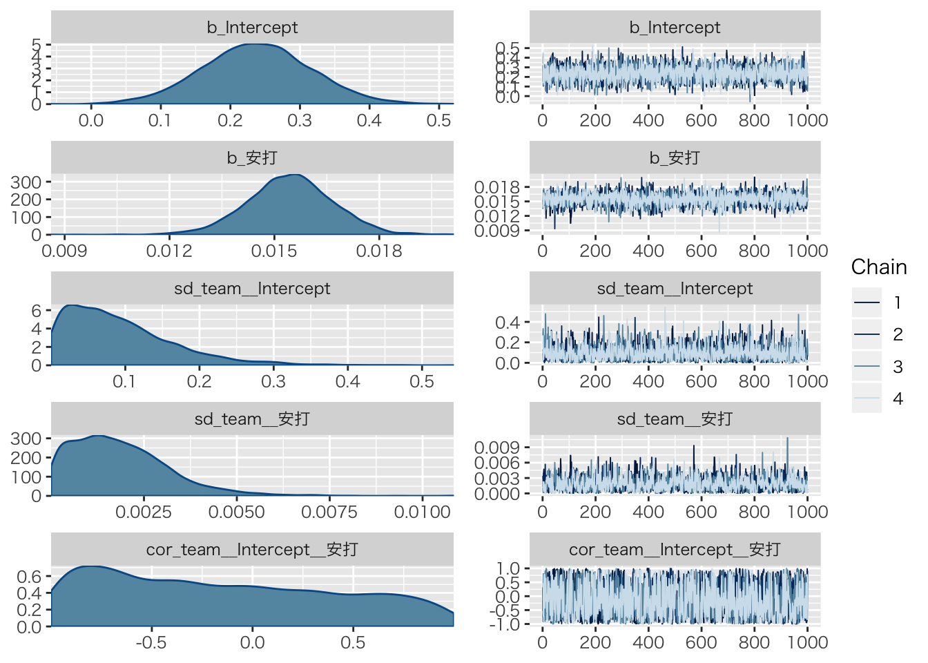

pp_check(result.hlm2)

## Using 10 posterior samples for ppc type 'dens_overlay' by default.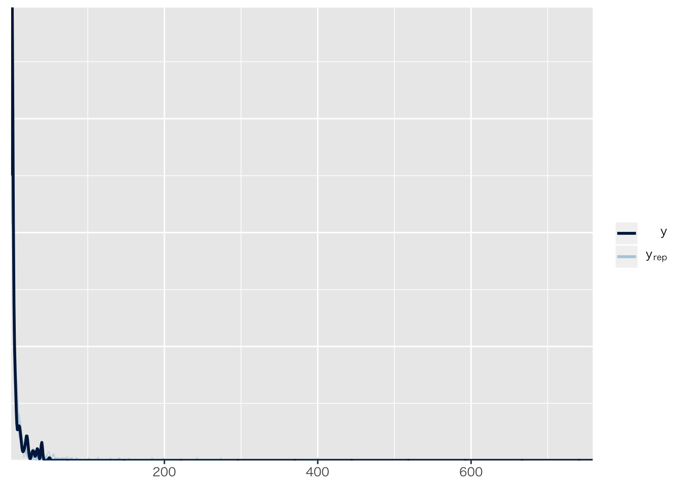

baseball_dat10 %>% 
  dplyr::select(salary,安打,team) %>% 
  na.omit() %>% 
  # 予測値をデータに追加
  cbind(fitted(result.hlm2)) %>% 
  ggplot(aes(安打, Estimate, color = team)) +
  geom_smooth(method = "lm", se = FALSE) +
  geom_point(aes(y = salary))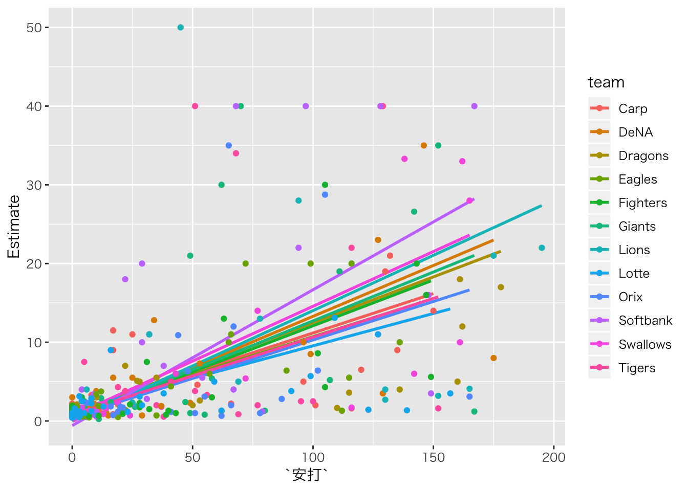

線形モデル6；分散分析と線形モデル

Between Design

「とあるスナック菓子を三人のこどもそれぞれに買い与えたが，お菓子の長さに差があると言って喧嘩を始めた。彼らの主張が妥当かどうか検証するために，それぞれの菓子袋から棒状のお菓子10本ずつをサンプリンングし，長さを測定した。三つの菓子袋に含まれるお菓子の長さに差があると言って良いかどうか，統計的に検定しなさい。」

id	group	L
1	A	9
2	A	7
3	A	8
4	A	5
5	A	9
6	B	12
7	B	10
8	B	23
9	B	19
10	B	16
11	C	9
12	C	16
13	C	16
14	C	14
15	C	5

## 
## [ As-Type Design ]
## 
## This output was generated by anovakun 4.8.2 under R version 3.5.2.
## It was executed on Fri Mar  8 17:06:46 2019.
## 
##  
## << DESCRIPTIVE STATISTICS >>
## 
## ---------------------------
##   A   n     Mean    S.D. 
## ---------------------------
##  a1   5   7.6000  1.6733 
##  a2   5  16.0000  5.2440 
##  a3   5  12.0000  4.8477 
## ---------------------------
## 
## 
## << ANOVA TABLE >>
## 
## -------------------------------------------------------
##  Source        SS  df       MS  F-ratio  p-value     
## -------------------------------------------------------
##       A  176.5333   2  88.2667   4.9219   0.0275 *   
##   Error  215.2000  12  17.9333                       
## -------------------------------------------------------
##   Total  391.7333  14  27.9810                       
##            +p < .10, *p < .05, **p < .01, ***p < .001
## 
## 
## << POST ANALYSES >>
## 
## < MULTIPLE COMPARISON for "A" >
## 
## == Shaffer's Modified Sequentially Rejective Bonferroni Procedure ==
## == The factor < A > is analysed as independent means. == 
## == Alpha level is 0.05. == 
##  
## ---------------------------
##   A   n     Mean    S.D. 
## ---------------------------
##  a1   5   7.6000  1.6733 
##  a2   5  16.0000  5.2440 
##  a3   5  12.0000  4.8477 
## ---------------------------
## 
## ----------------------------------------------------------
##   Pair     Diff  t-value  df       p   adj.p            
## ----------------------------------------------------------
##  a1-a2  -8.4000   3.1363  12  0.0086  0.0258  a1 < a2 * 
##  a1-a3  -4.4000   1.6428  12  0.1263  0.1263  a1 = a3   
##  a2-a3   4.0000   1.4935  12  0.1611  0.1611  a2 = a3   
## ----------------------------------------------------------
## 
## 
## output is over --------------------///

線形モデルの文脈で。

result.anova1 <- brm(L~group,data=dat)

## Compiling the C++ model

## Start sampling

## 
## SAMPLING FOR MODEL 'd8d7c25c08bf7eeac588d635c6649298' NOW (CHAIN 1).
## Chain 1: 
## Chain 1: Gradient evaluation took 3.2e-05 seconds
## Chain 1: 1000 transitions using 10 leapfrog steps per transition would take 0.32 seconds.
## Chain 1: Adjust your expectations accordingly!
## Chain 1: 
## Chain 1: 
## Chain 1: Iteration:    1 / 2000 [  0%]  (Warmup)
## Chain 1: Iteration:  200 / 2000 [ 10%]  (Warmup)
## Chain 1: Iteration:  400 / 2000 [ 20%]  (Warmup)
## Chain 1: Iteration:  600 / 2000 [ 30%]  (Warmup)
## Chain 1: Iteration:  800 / 2000 [ 40%]  (Warmup)
## Chain 1: Iteration: 1000 / 2000 [ 50%]  (Warmup)
## Chain 1: Iteration: 1001 / 2000 [ 50%]  (Sampling)
## Chain 1: Iteration: 1200 / 2000 [ 60%]  (Sampling)
## Chain 1: Iteration: 1400 / 2000 [ 70%]  (Sampling)
## Chain 1: Iteration: 1600 / 2000 [ 80%]  (Sampling)
## Chain 1: Iteration: 1800 / 2000 [ 90%]  (Sampling)
## Chain 1: Iteration: 2000 / 2000 [100%]  (Sampling)
## Chain 1: 
## Chain 1:  Elapsed Time: 0.064369 seconds (Warm-up)
## Chain 1:                0.045909 seconds (Sampling)
## Chain 1:                0.110278 seconds (Total)
## Chain 1: 
## 
## SAMPLING FOR MODEL 'd8d7c25c08bf7eeac588d635c6649298' NOW (CHAIN 2).
## Chain 2: 
## Chain 2: Gradient evaluation took 1.1e-05 seconds
## Chain 2: 1000 transitions using 10 leapfrog steps per transition would take 0.11 seconds.
## Chain 2: Adjust your expectations accordingly!
## Chain 2: 
## Chain 2: 
## Chain 2: Iteration:    1 / 2000 [  0%]  (Warmup)
## Chain 2: Iteration:  200 / 2000 [ 10%]  (Warmup)
## Chain 2: Iteration:  400 / 2000 [ 20%]  (Warmup)
## Chain 2: Iteration:  600 / 2000 [ 30%]  (Warmup)
## Chain 2: Iteration:  800 / 2000 [ 40%]  (Warmup)
## Chain 2: Iteration: 1000 / 2000 [ 50%]  (Warmup)
## Chain 2: Iteration: 1001 / 2000 [ 50%]  (Sampling)
## Chain 2: Iteration: 1200 / 2000 [ 60%]  (Sampling)
## Chain 2: Iteration: 1400 / 2000 [ 70%]  (Sampling)
## Chain 2: Iteration: 1600 / 2000 [ 80%]  (Sampling)
## Chain 2: Iteration: 1800 / 2000 [ 90%]  (Sampling)
## Chain 2: Iteration: 2000 / 2000 [100%]  (Sampling)
## Chain 2: 
## Chain 2:  Elapsed Time: 0.063472 seconds (Warm-up)
## Chain 2:                0.045855 seconds (Sampling)
## Chain 2:                0.109327 seconds (Total)
## Chain 2: 
## 
## SAMPLING FOR MODEL 'd8d7c25c08bf7eeac588d635c6649298' NOW (CHAIN 3).
## Chain 3: 
## Chain 3: Gradient evaluation took 1.2e-05 seconds
## Chain 3: 1000 transitions using 10 leapfrog steps per transition would take 0.12 seconds.
## Chain 3: Adjust your expectations accordingly!
## Chain 3: 
## Chain 3: 
## Chain 3: Iteration:    1 / 2000 [  0%]  (Warmup)
## Chain 3: Iteration:  200 / 2000 [ 10%]  (Warmup)
## Chain 3: Iteration:  400 / 2000 [ 20%]  (Warmup)
## Chain 3: Iteration:  600 / 2000 [ 30%]  (Warmup)
## Chain 3: Iteration:  800 / 2000 [ 40%]  (Warmup)
## Chain 3: Iteration: 1000 / 2000 [ 50%]  (Warmup)
## Chain 3: Iteration: 1001 / 2000 [ 50%]  (Sampling)
## Chain 3: Iteration: 1200 / 2000 [ 60%]  (Sampling)
## Chain 3: Iteration: 1400 / 2000 [ 70%]  (Sampling)
## Chain 3: Iteration: 1600 / 2000 [ 80%]  (Sampling)
## Chain 3: Iteration: 1800 / 2000 [ 90%]  (Sampling)
## Chain 3: Iteration: 2000 / 2000 [100%]  (Sampling)
## Chain 3: 
## Chain 3:  Elapsed Time: 0.068084 seconds (Warm-up)
## Chain 3:                0.043967 seconds (Sampling)
## Chain 3:                0.112051 seconds (Total)
## Chain 3: 
## 
## SAMPLING FOR MODEL 'd8d7c25c08bf7eeac588d635c6649298' NOW (CHAIN 4).
## Chain 4: 
## Chain 4: Gradient evaluation took 1e-05 seconds
## Chain 4: 1000 transitions using 10 leapfrog steps per transition would take 0.1 seconds.
## Chain 4: Adjust your expectations accordingly!
## Chain 4: 
## Chain 4: 
## Chain 4: Iteration:    1 / 2000 [  0%]  (Warmup)
## Chain 4: Iteration:  200 / 2000 [ 10%]  (Warmup)
## Chain 4: Iteration:  400 / 2000 [ 20%]  (Warmup)
## Chain 4: Iteration:  600 / 2000 [ 30%]  (Warmup)
## Chain 4: Iteration:  800 / 2000 [ 40%]  (Warmup)
## Chain 4: Iteration: 1000 / 2000 [ 50%]  (Warmup)
## Chain 4: Iteration: 1001 / 2000 [ 50%]  (Sampling)
## Chain 4: Iteration: 1200 / 2000 [ 60%]  (Sampling)
## Chain 4: Iteration: 1400 / 2000 [ 70%]  (Sampling)
## Chain 4: Iteration: 1600 / 2000 [ 80%]  (Sampling)
## Chain 4: Iteration: 1800 / 2000 [ 90%]  (Sampling)
## Chain 4: Iteration: 2000 / 2000 [100%]  (Sampling)
## Chain 4: 
## Chain 4:  Elapsed Time: 0.073345 seconds (Warm-up)
## Chain 4:                0.054849 seconds (Sampling)
## Chain 4:                0.128194 seconds (Total)
## Chain 4:

result.anova1

##  Family: gaussian 
##   Links: mu = identity; sigma = identity 
## Formula: L ~ group 
##    Data: dat (Number of observations: 15) 
## Samples: 4 chains, each with iter = 2000; warmup = 1000; thin = 1;
##          total post-warmup samples = 4000
## 
## Population-Level Effects: 
##           Estimate Est.Error l-95% CI u-95% CI Eff.Sample Rhat
## Intercept     7.56      2.19     3.32    12.00       3028 1.00
## groupB        8.43      3.08     2.29    14.49       3382 1.00
## groupC        4.35      2.99    -1.65    10.48       3125 1.00
## 
## Family Specific Parameters: 
##       Estimate Est.Error l-95% CI u-95% CI Eff.Sample Rhat
## sigma     4.67      1.04     3.21     7.15       2310 1.00
## 
## Samples were drawn using sampling(NUTS). For each parameter, Eff.Sample 
## is a crude measure of effective sample size, and Rhat is the potential 
## scale reduction factor on split chains (at convergence, Rhat = 1).

plot(marginal_effects(result.anova1))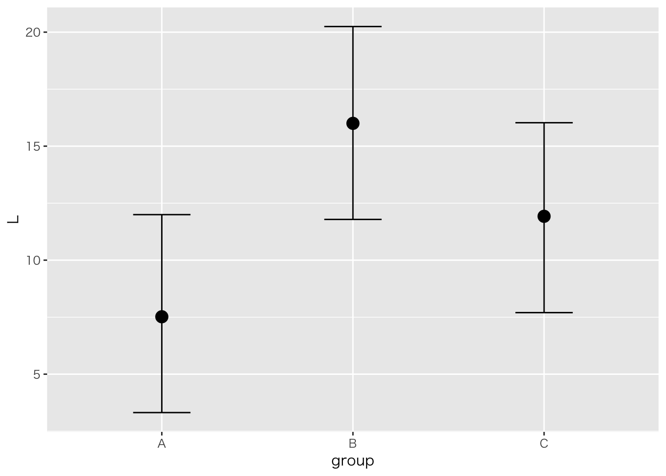

##### モデル比較

result.anova1.null <- brm(L~1,data=dat)

## Compiling the C++ model

## Start sampling

## 
## SAMPLING FOR MODEL '65e149dd8c76fca577ab92d97eef3fd8' NOW (CHAIN 1).
## Chain 1: 
## Chain 1: Gradient evaluation took 1.9e-05 seconds
## Chain 1: 1000 transitions using 10 leapfrog steps per transition would take 0.19 seconds.
## Chain 1: Adjust your expectations accordingly!
## Chain 1: 
## Chain 1: 
## Chain 1: Iteration:    1 / 2000 [  0%]  (Warmup)
## Chain 1: Iteration:  200 / 2000 [ 10%]  (Warmup)
## Chain 1: Iteration:  400 / 2000 [ 20%]  (Warmup)
## Chain 1: Iteration:  600 / 2000 [ 30%]  (Warmup)
## Chain 1: Iteration:  800 / 2000 [ 40%]  (Warmup)
## Chain 1: Iteration: 1000 / 2000 [ 50%]  (Warmup)
## Chain 1: Iteration: 1001 / 2000 [ 50%]  (Sampling)
## Chain 1: Iteration: 1200 / 2000 [ 60%]  (Sampling)
## Chain 1: Iteration: 1400 / 2000 [ 70%]  (Sampling)
## Chain 1: Iteration: 1600 / 2000 [ 80%]  (Sampling)
## Chain 1: Iteration: 1800 / 2000 [ 90%]  (Sampling)
## Chain 1: Iteration: 2000 / 2000 [100%]  (Sampling)
## Chain 1: 
## Chain 1:  Elapsed Time: 0.030212 seconds (Warm-up)
## Chain 1:                0.037674 seconds (Sampling)
## Chain 1:                0.067886 seconds (Total)
## Chain 1: 
## 
## SAMPLING FOR MODEL '65e149dd8c76fca577ab92d97eef3fd8' NOW (CHAIN 2).
## Chain 2: 
## Chain 2: Gradient evaluation took 9e-06 seconds
## Chain 2: 1000 transitions using 10 leapfrog steps per transition would take 0.09 seconds.
## Chain 2: Adjust your expectations accordingly!
## Chain 2: 
## Chain 2: 
## Chain 2: Iteration:    1 / 2000 [  0%]  (Warmup)
## Chain 2: Iteration:  200 / 2000 [ 10%]  (Warmup)
## Chain 2: Iteration:  400 / 2000 [ 20%]  (Warmup)
## Chain 2: Iteration:  600 / 2000 [ 30%]  (Warmup)
## Chain 2: Iteration:  800 / 2000 [ 40%]  (Warmup)
## Chain 2: Iteration: 1000 / 2000 [ 50%]  (Warmup)
## Chain 2: Iteration: 1001 / 2000 [ 50%]  (Sampling)
## Chain 2: Iteration: 1200 / 2000 [ 60%]  (Sampling)
## Chain 2: Iteration: 1400 / 2000 [ 70%]  (Sampling)
## Chain 2: Iteration: 1600 / 2000 [ 80%]  (Sampling)
## Chain 2: Iteration: 1800 / 2000 [ 90%]  (Sampling)
## Chain 2: Iteration: 2000 / 2000 [100%]  (Sampling)
## Chain 2: 
## Chain 2:  Elapsed Time: 0.031314 seconds (Warm-up)
## Chain 2:                0.027261 seconds (Sampling)
## Chain 2:                0.058575 seconds (Total)
## Chain 2: 
## 
## SAMPLING FOR MODEL '65e149dd8c76fca577ab92d97eef3fd8' NOW (CHAIN 3).
## Chain 3: 
## Chain 3: Gradient evaluation took 9e-06 seconds
## Chain 3: 1000 transitions using 10 leapfrog steps per transition would take 0.09 seconds.
## Chain 3: Adjust your expectations accordingly!
## Chain 3: 
## Chain 3: 
## Chain 3: Iteration:    1 / 2000 [  0%]  (Warmup)
## Chain 3: Iteration:  200 / 2000 [ 10%]  (Warmup)
## Chain 3: Iteration:  400 / 2000 [ 20%]  (Warmup)
## Chain 3: Iteration:  600 / 2000 [ 30%]  (Warmup)
## Chain 3: Iteration:  800 / 2000 [ 40%]  (Warmup)
## Chain 3: Iteration: 1000 / 2000 [ 50%]  (Warmup)
## Chain 3: Iteration: 1001 / 2000 [ 50%]  (Sampling)
## Chain 3: Iteration: 1200 / 2000 [ 60%]  (Sampling)
## Chain 3: Iteration: 1400 / 2000 [ 70%]  (Sampling)
## Chain 3: Iteration: 1600 / 2000 [ 80%]  (Sampling)
## Chain 3: Iteration: 1800 / 2000 [ 90%]  (Sampling)
## Chain 3: Iteration: 2000 / 2000 [100%]  (Sampling)
## Chain 3: 
## Chain 3:  Elapsed Time: 0.031735 seconds (Warm-up)
## Chain 3:                0.027487 seconds (Sampling)
## Chain 3:                0.059222 seconds (Total)
## Chain 3: 
## 
## SAMPLING FOR MODEL '65e149dd8c76fca577ab92d97eef3fd8' NOW (CHAIN 4).
## Chain 4: 
## Chain 4: Gradient evaluation took 7e-06 seconds
## Chain 4: 1000 transitions using 10 leapfrog steps per transition would take 0.07 seconds.
## Chain 4: Adjust your expectations accordingly!
## Chain 4: 
## Chain 4: 
## Chain 4: Iteration:    1 / 2000 [  0%]  (Warmup)
## Chain 4: Iteration:  200 / 2000 [ 10%]  (Warmup)
## Chain 4: Iteration:  400 / 2000 [ 20%]  (Warmup)
## Chain 4: Iteration:  600 / 2000 [ 30%]  (Warmup)
## Chain 4: Iteration:  800 / 2000 [ 40%]  (Warmup)
## Chain 4: Iteration: 1000 / 2000 [ 50%]  (Warmup)
## Chain 4: Iteration: 1001 / 2000 [ 50%]  (Sampling)
## Chain 4: Iteration: 1200 / 2000 [ 60%]  (Sampling)
## Chain 4: Iteration: 1400 / 2000 [ 70%]  (Sampling)
## Chain 4: Iteration: 1600 / 2000 [ 80%]  (Sampling)
## Chain 4: Iteration: 1800 / 2000 [ 90%]  (Sampling)
## Chain 4: Iteration: 2000 / 2000 [100%]  (Sampling)
## Chain 4: 
## Chain 4:  Elapsed Time: 0.029459 seconds (Warm-up)
## Chain 4:                0.026404 seconds (Sampling)
## Chain 4:                0.055863 seconds (Total)
## Chain 4:

result.anova1.null

##  Family: gaussian 
##   Links: mu = identity; sigma = identity 
## Formula: L ~ 1 
##    Data: dat (Number of observations: 15) 
## Samples: 4 chains, each with iter = 2000; warmup = 1000; thin = 1;
##          total post-warmup samples = 4000
## 
## Population-Level Effects: 
##           Estimate Est.Error l-95% CI u-95% CI Eff.Sample Rhat
## Intercept    11.79      1.45     8.89    14.62       2633 1.00
## 
## Family Specific Parameters: 
##       Estimate Est.Error l-95% CI u-95% CI Eff.Sample Rhat
## sigma     5.70      1.15     4.01     8.33       2515 1.00
## 
## Samples were drawn using sampling(NUTS). For each parameter, Eff.Sample 
## is a crude measure of effective sample size, and Rhat is the potential 
## scale reduction factor on split chains (at convergence, Rhat = 1).

# モデル比較
brms::WAIC(result.anova1,result.anova1.null)

##                                     WAIC   SE
## result.anova1                      90.83 4.28
## result.anova1.null                 95.32 4.99
## result.anova1 - result.anova1.null -4.49 4.17

Within Design

内要因のデータは，個人で階層化されてるモデルと同じこと。

「自分の学級で前期，中期，後期に学力テストを行った。三回の学力テストは異なる設問だが難易度は同じぐらいであったとする。三つの時期で学力に違いがあると言って良いか，統計的に検定しなさい。」

## 
## [ sA-Type Design ]
## 
## This output was generated by anovakun 4.8.2 under R version 3.5.2.
## It was executed on Fri Mar  8 17:08:24 2019.
## 
##  
## << DESCRIPTIVE STATISTICS >>
## 
## ------------------------------
##    key   n     Mean    S.D. 
## ------------------------------
##  Time1  10  59.8000  7.3756 
##  Time2  10  67.5000  8.0450 
##  Time3  10  79.8000  4.4920 
## ------------------------------
## 
## 
## << SPHERICITY INDICES >>
## 
## == Mendoza's Multisample Sphericity Test and Epsilons ==
## 
## -------------------------------------------------------------------------
##  Effect  Lambda  approx.Chi  df      p         LB     GG     HF     CM 
## -------------------------------------------------------------------------
##     key  0.5333      1.1178   2 0.5718 ns  0.5000 0.8846 1.0851 0.9417 
## -------------------------------------------------------------------------
##                               LB = lower.bound, GG = Greenhouse-Geisser
##                              HF = Huynh-Feldt-Lecoutre, CM = Chi-Muller
## 
## 
## << ANOVA TABLE >>
## 
## -----------------------------------------------------------------
##  Source        SS  df        MS  F-ratio  p-value      p.eta^2 
## -----------------------------------------------------------------
##       s  559.6333   9   62.1815                                
## -----------------------------------------------------------------
##     key 2035.2667   2 1017.6333  26.3914   0.0000 ***   0.7457 
## s x key  694.0667  18   38.5593                                
## -----------------------------------------------------------------
##   Total 3288.9667  29  113.4126                                
##                      +p < .10, *p < .05, **p < .01, ***p < .001
## 
## 
## << POST ANALYSES >>
## 
## < MULTIPLE COMPARISON for "key" >
## 
## == Shaffer's Modified Sequentially Rejective Bonferroni Procedure ==
## == The factor < key > is analysed as dependent means. == 
## == Alpha level is 0.05. == 
##  
## ------------------------------
##    key   n     Mean    S.D. 
## ------------------------------
##  Time1  10  59.8000  7.3756 
##  Time2  10  67.5000  8.0450 
##  Time3  10  79.8000  4.4920 
## ------------------------------
## 
## -----------------------------------------------------------------------
##         Pair      Diff  t-value  df       p   adj.p                  
## -----------------------------------------------------------------------
##  Time1-Time3  -20.0000   8.0611   9  0.0000  0.0001  Time1 < Time3 * 
##  Time2-Time3  -12.3000   3.7977   9  0.0042  0.0042  Time2 < Time3 * 
##  Time1-Time2   -7.7000   3.0225   9  0.0144  0.0144  Time1 < Time2 * 
## -----------------------------------------------------------------------
## 
## 
## output is over --------------------///

線形モデルとして。

result.anova2 <- brm(val~key+(1|ID),data=dat2)

## Compiling the C++ model

## Start sampling

## 
## SAMPLING FOR MODEL '0de9cd3fd8b99f21ecd5fa335f74897b' NOW (CHAIN 1).
## Chain 1: 
## Chain 1: Gradient evaluation took 5.1e-05 seconds
## Chain 1: 1000 transitions using 10 leapfrog steps per transition would take 0.51 seconds.
## Chain 1: Adjust your expectations accordingly!
## Chain 1: 
## Chain 1: 
## Chain 1: Iteration:    1 / 2000 [  0%]  (Warmup)
## Chain 1: Iteration:  200 / 2000 [ 10%]  (Warmup)
## Chain 1: Iteration:  400 / 2000 [ 20%]  (Warmup)
## Chain 1: Iteration:  600 / 2000 [ 30%]  (Warmup)
## Chain 1: Iteration:  800 / 2000 [ 40%]  (Warmup)
## Chain 1: Iteration: 1000 / 2000 [ 50%]  (Warmup)
## Chain 1: Iteration: 1001 / 2000 [ 50%]  (Sampling)
## Chain 1: Iteration: 1200 / 2000 [ 60%]  (Sampling)
## Chain 1: Iteration: 1400 / 2000 [ 70%]  (Sampling)
## Chain 1: Iteration: 1600 / 2000 [ 80%]  (Sampling)
## Chain 1: Iteration: 1800 / 2000 [ 90%]  (Sampling)
## Chain 1: Iteration: 2000 / 2000 [100%]  (Sampling)
## Chain 1: 
## Chain 1:  Elapsed Time: 0.214928 seconds (Warm-up)
## Chain 1:                0.163653 seconds (Sampling)
## Chain 1:                0.378581 seconds (Total)
## Chain 1: 
## 
## SAMPLING FOR MODEL '0de9cd3fd8b99f21ecd5fa335f74897b' NOW (CHAIN 2).
## Chain 2: 
## Chain 2: Gradient evaluation took 1.9e-05 seconds
## Chain 2: 1000 transitions using 10 leapfrog steps per transition would take 0.19 seconds.
## Chain 2: Adjust your expectations accordingly!
## Chain 2: 
## Chain 2: 
## Chain 2: Iteration:    1 / 2000 [  0%]  (Warmup)
## Chain 2: Iteration:  200 / 2000 [ 10%]  (Warmup)
## Chain 2: Iteration:  400 / 2000 [ 20%]  (Warmup)
## Chain 2: Iteration:  600 / 2000 [ 30%]  (Warmup)
## Chain 2: Iteration:  800 / 2000 [ 40%]  (Warmup)
## Chain 2: Iteration: 1000 / 2000 [ 50%]  (Warmup)
## Chain 2: Iteration: 1001 / 2000 [ 50%]  (Sampling)
## Chain 2: Iteration: 1200 / 2000 [ 60%]  (Sampling)
## Chain 2: Iteration: 1400 / 2000 [ 70%]  (Sampling)
## Chain 2: Iteration: 1600 / 2000 [ 80%]  (Sampling)
## Chain 2: Iteration: 1800 / 2000 [ 90%]  (Sampling)
## Chain 2: Iteration: 2000 / 2000 [100%]  (Sampling)
## Chain 2: 
## Chain 2:  Elapsed Time: 0.215893 seconds (Warm-up)
## Chain 2:                0.168583 seconds (Sampling)
## Chain 2:                0.384476 seconds (Total)
## Chain 2: 
## 
## SAMPLING FOR MODEL '0de9cd3fd8b99f21ecd5fa335f74897b' NOW (CHAIN 3).
## Chain 3: 
## Chain 3: Gradient evaluation took 2e-05 seconds
## Chain 3: 1000 transitions using 10 leapfrog steps per transition would take 0.2 seconds.
## Chain 3: Adjust your expectations accordingly!
## Chain 3: 
## Chain 3: 
## Chain 3: Iteration:    1 / 2000 [  0%]  (Warmup)
## Chain 3: Iteration:  200 / 2000 [ 10%]  (Warmup)
## Chain 3: Iteration:  400 / 2000 [ 20%]  (Warmup)
## Chain 3: Iteration:  600 / 2000 [ 30%]  (Warmup)
## Chain 3: Iteration:  800 / 2000 [ 40%]  (Warmup)
## Chain 3: Iteration: 1000 / 2000 [ 50%]  (Warmup)
## Chain 3: Iteration: 1001 / 2000 [ 50%]  (Sampling)
## Chain 3: Iteration: 1200 / 2000 [ 60%]  (Sampling)
## Chain 3: Iteration: 1400 / 2000 [ 70%]  (Sampling)
## Chain 3: Iteration: 1600 / 2000 [ 80%]  (Sampling)
## Chain 3: Iteration: 1800 / 2000 [ 90%]  (Sampling)
## Chain 3: Iteration: 2000 / 2000 [100%]  (Sampling)
## Chain 3: 
## Chain 3:  Elapsed Time: 0.229098 seconds (Warm-up)
## Chain 3:                0.171995 seconds (Sampling)
## Chain 3:                0.401093 seconds (Total)
## Chain 3: 
## 
## SAMPLING FOR MODEL '0de9cd3fd8b99f21ecd5fa335f74897b' NOW (CHAIN 4).
## Chain 4: 
## Chain 4: Gradient evaluation took 1.9e-05 seconds
## Chain 4: 1000 transitions using 10 leapfrog steps per transition would take 0.19 seconds.
## Chain 4: Adjust your expectations accordingly!
## Chain 4: 
## Chain 4: 
## Chain 4: Iteration:    1 / 2000 [  0%]  (Warmup)
## Chain 4: Iteration:  200 / 2000 [ 10%]  (Warmup)
## Chain 4: Iteration:  400 / 2000 [ 20%]  (Warmup)
## Chain 4: Iteration:  600 / 2000 [ 30%]  (Warmup)
## Chain 4: Iteration:  800 / 2000 [ 40%]  (Warmup)
## Chain 4: Iteration: 1000 / 2000 [ 50%]  (Warmup)
## Chain 4: Iteration: 1001 / 2000 [ 50%]  (Sampling)
## Chain 4: Iteration: 1200 / 2000 [ 60%]  (Sampling)
## Chain 4: Iteration: 1400 / 2000 [ 70%]  (Sampling)
## Chain 4: Iteration: 1600 / 2000 [ 80%]  (Sampling)
## Chain 4: Iteration: 1800 / 2000 [ 90%]  (Sampling)
## Chain 4: Iteration: 2000 / 2000 [100%]  (Sampling)
## Chain 4: 
## Chain 4:  Elapsed Time: 0.244533 seconds (Warm-up)
## Chain 4:                0.164979 seconds (Sampling)
## Chain 4:                0.409512 seconds (Total)
## Chain 4:

result.anova2

##  Family: gaussian 
##   Links: mu = identity; sigma = identity 
## Formula: val ~ key + (1 | ID) 
##    Data: dat2 (Number of observations: 30) 
## Samples: 4 chains, each with iter = 2000; warmup = 1000; thin = 1;
##          total post-warmup samples = 4000
## 
## Group-Level Effects: 
## ~ID (Number of levels: 10) 
##               Estimate Est.Error l-95% CI u-95% CI Eff.Sample Rhat
## sd(Intercept)     3.12      1.91     0.22     7.46       1200 1.00
## 
## Population-Level Effects: 
##           Estimate Est.Error l-95% CI u-95% CI Eff.Sample Rhat
## Intercept    59.80      2.43    54.88    64.59       2505 1.00
## keyTime2      7.76      2.97     2.07    13.74       3308 1.00
## keyTime3     20.07      2.97    14.23    26.05       3202 1.00
## 
## Family Specific Parameters: 
##       Estimate Est.Error l-95% CI u-95% CI Eff.Sample Rhat
## sigma     6.53      1.03     4.79     8.82       2368 1.00
## 
## Samples were drawn using sampling(NUTS). For each parameter, Eff.Sample 
## is a crude measure of effective sample size, and Rhat is the potential 
## scale reduction factor on split chains (at convergence, Rhat = 1).

plot(marginal_effects(result.anova2))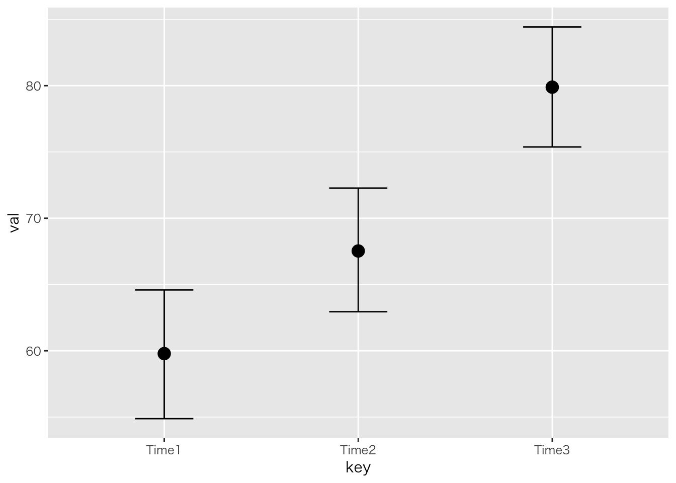

ggplot(dat2,aes(x=key,y=val,color=ID,group=ID))+geom_point()+
  geom_smooth(method="lm",se=F)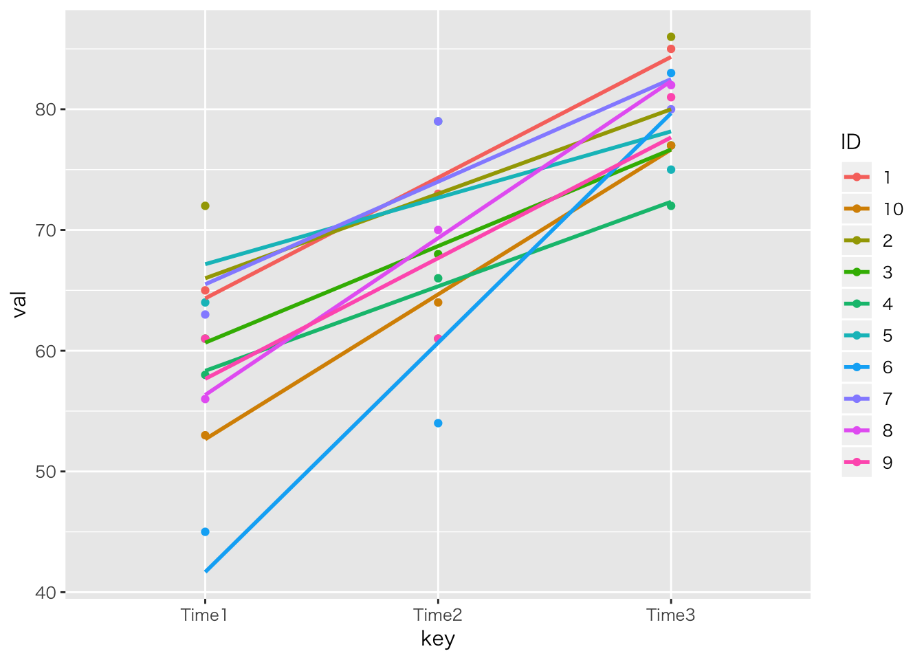

Mixed Design

「ある学校では二種類のテキストを使って，どちらが成績に良い影響を与えるか検証した。テキストはA1,A2の二種類であり，成績は前後の二回で比較する。５人ずつの学級で検証した。テキストの効果，成績の上昇はあると言って良いか統計的に検定せよ」

ID	Text	pre	post
1	A1	78	45
2	A1	76	47
3	A1	72	31
4	A1	61	36
5	A1	69	44
6	A2	24	60
7	A2	44	86
8	A2	29	58
9	A2	24	60
10	A2	37	68

## 
## [ AsB-Type Design ]
## 
## This output was generated by anovakun 4.8.2 under R version 3.5.2.
## It was executed on Fri Mar  8 17:09:17 2019.
## 
##  
## << DESCRIPTIVE STATISTICS >>
## 
## --------------------------------
##   A   B   n     Mean     S.D. 
## --------------------------------
##  a1  b1   5  71.2000   6.6858 
##  a1  b2   5  40.6000   6.8044 
##  a2  b1   5  31.6000   8.7350 
##  a2  b2   5  66.4000  11.6103 
## --------------------------------
## 
## 
## << SPHERICITY INDICES >>
## 
## == Mendoza's Multisample Sphericity Test and Epsilons ==
## 
## -------------------------------------------------------------------------
##  Effect  Lambda  approx.Chi  df      p         LB     GG     HF     CM 
## -------------------------------------------------------------------------
##       B  0.8586      0.2668   1 0.6055 ns  1.0000 1.0000 1.0000 1.0000 
## -------------------------------------------------------------------------
##                               LB = lower.bound, GG = Greenhouse-Geisser
##                              HF = Huynh-Feldt-Lecoutre, CM = Chi-Muller
## 
## 
## << ANOVA TABLE >>
## 
## ---------------------------------------------------------------
##     Source         SS  df         MS   F-ratio  p-value      
## ---------------------------------------------------------------
##          A   238.0500   1   238.0500    1.7841   0.2184 ns   
##      s x A  1067.4000   8   133.4250                         
## ---------------------------------------------------------------
##          B    22.0500   1    22.0500    1.2511   0.2958 ns   
##      A x B  5346.4500   1  5346.4500  303.3447   0.0000 ***  
##  s x A x B   141.0000   8    17.6250                         
## ---------------------------------------------------------------
##      Total  6814.9500  19   358.6816                         
##                    +p < .10, *p < .05, **p < .01, ***p < .001
## 
## 
## << POST ANALYSES >>
## 
## < SIMPLE EFFECTS for "A x B" INTERACTION >
## 
## -----------------------------------------------------------------------
##   Effect  Lambda  approx.Chi  df   p         LB     GG     HF     CM 
## -----------------------------------------------------------------------
##  B at a1  1.0000     -0.0000   0         1.0000 1.0000 1.0000 1.0000 
##  B at a2  1.0000     -0.0000   0         1.0000 1.0000 1.0000 1.0000 
## -----------------------------------------------------------------------
##                             LB = lower.bound, GG = Greenhouse-Geisser
##                            HF = Huynh-Feldt-Lecoutre, CM = Chi-Muller
## 
## -----------------------------------------------------------------
##       Source         SS  df         MS   F-ratio  p-value      
## -----------------------------------------------------------------
##      A at b1  3920.4000   1  3920.4000   64.8000   0.0000 ***  
##     Er at b1   484.0000   8    60.5000                         
## -----------------------------------------------------------------
##      A at b2  1664.1000   1  1664.1000   18.3777   0.0027 **   
##     Er at b2   724.4000   8    90.5500                         
## -----------------------------------------------------------------
##      B at a1  2340.9000   1  2340.9000  104.5045   0.0005 ***  
##  s x B at a1    89.6000   4    22.4000                         
## -----------------------------------------------------------------
##      B at a2  3027.6000   1  3027.6000  235.6109   0.0001 ***  
##  s x B at a2    51.4000   4    12.8500                         
## -----------------------------------------------------------------
##                      +p < .10, *p < .05, **p < .01, ***p < .001
## 
## output is over --------------------///

線形モデルとして。

dat %>% 
  tidyr::gather(key,val,-ID,-Text,factor_key=TRUE) -> dat3

result.anova3 <- brm(val~Text*key + (1|ID),data=dat3)

## Compiling the C++ model

## Start sampling

## 
## SAMPLING FOR MODEL 'be967cbea7bb3bc2f2e9f7b9c0e66a66' NOW (CHAIN 1).
## Chain 1: 
## Chain 1: Gradient evaluation took 5.3e-05 seconds
## Chain 1: 1000 transitions using 10 leapfrog steps per transition would take 0.53 seconds.
## Chain 1: Adjust your expectations accordingly!
## Chain 1: 
## Chain 1: 
## Chain 1: Iteration:    1 / 2000 [  0%]  (Warmup)
## Chain 1: Iteration:  200 / 2000 [ 10%]  (Warmup)
## Chain 1: Iteration:  400 / 2000 [ 20%]  (Warmup)
## Chain 1: Iteration:  600 / 2000 [ 30%]  (Warmup)
## Chain 1: Iteration:  800 / 2000 [ 40%]  (Warmup)
## Chain 1: Iteration: 1000 / 2000 [ 50%]  (Warmup)
## Chain 1: Iteration: 1001 / 2000 [ 50%]  (Sampling)
## Chain 1: Iteration: 1200 / 2000 [ 60%]  (Sampling)
## Chain 1: Iteration: 1400 / 2000 [ 70%]  (Sampling)
## Chain 1: Iteration: 1600 / 2000 [ 80%]  (Sampling)
## Chain 1: Iteration: 1800 / 2000 [ 90%]  (Sampling)
## Chain 1: Iteration: 2000 / 2000 [100%]  (Sampling)
## Chain 1: 
## Chain 1:  Elapsed Time: 0.314932 seconds (Warm-up)
## Chain 1:                0.167302 seconds (Sampling)
## Chain 1:                0.482234 seconds (Total)
## Chain 1: 
## 
## SAMPLING FOR MODEL 'be967cbea7bb3bc2f2e9f7b9c0e66a66' NOW (CHAIN 2).
## Chain 2: 
## Chain 2: Gradient evaluation took 2.3e-05 seconds
## Chain 2: 1000 transitions using 10 leapfrog steps per transition would take 0.23 seconds.
## Chain 2: Adjust your expectations accordingly!
## Chain 2: 
## Chain 2: 
## Chain 2: Iteration:    1 / 2000 [  0%]  (Warmup)
## Chain 2: Iteration:  200 / 2000 [ 10%]  (Warmup)
## Chain 2: Iteration:  400 / 2000 [ 20%]  (Warmup)
## Chain 2: Iteration:  600 / 2000 [ 30%]  (Warmup)
## Chain 2: Iteration:  800 / 2000 [ 40%]  (Warmup)
## Chain 2: Iteration: 1000 / 2000 [ 50%]  (Warmup)
## Chain 2: Iteration: 1001 / 2000 [ 50%]  (Sampling)
## Chain 2: Iteration: 1200 / 2000 [ 60%]  (Sampling)
## Chain 2: Iteration: 1400 / 2000 [ 70%]  (Sampling)
## Chain 2: Iteration: 1600 / 2000 [ 80%]  (Sampling)
## Chain 2: Iteration: 1800 / 2000 [ 90%]  (Sampling)
## Chain 2: Iteration: 2000 / 2000 [100%]  (Sampling)
## Chain 2: 
## Chain 2:  Elapsed Time: 0.326233 seconds (Warm-up)
## Chain 2:                0.253915 seconds (Sampling)
## Chain 2:                0.580148 seconds (Total)
## Chain 2: 
## 
## SAMPLING FOR MODEL 'be967cbea7bb3bc2f2e9f7b9c0e66a66' NOW (CHAIN 3).
## Chain 3: 
## Chain 3: Gradient evaluation took 3.4e-05 seconds
## Chain 3: 1000 transitions using 10 leapfrog steps per transition would take 0.34 seconds.
## Chain 3: Adjust your expectations accordingly!
## Chain 3: 
## Chain 3: 
## Chain 3: Iteration:    1 / 2000 [  0%]  (Warmup)
## Chain 3: Iteration:  200 / 2000 [ 10%]  (Warmup)
## Chain 3: Iteration:  400 / 2000 [ 20%]  (Warmup)
## Chain 3: Iteration:  600 / 2000 [ 30%]  (Warmup)
## Chain 3: Iteration:  800 / 2000 [ 40%]  (Warmup)
## Chain 3: Iteration: 1000 / 2000 [ 50%]  (Warmup)
## Chain 3: Iteration: 1001 / 2000 [ 50%]  (Sampling)
## Chain 3: Iteration: 1200 / 2000 [ 60%]  (Sampling)
## Chain 3: Iteration: 1400 / 2000 [ 70%]  (Sampling)
## Chain 3: Iteration: 1600 / 2000 [ 80%]  (Sampling)
## Chain 3: Iteration: 1800 / 2000 [ 90%]  (Sampling)
## Chain 3: Iteration: 2000 / 2000 [100%]  (Sampling)
## Chain 3: 
## Chain 3:  Elapsed Time: 0.351362 seconds (Warm-up)
## Chain 3:                0.237883 seconds (Sampling)
## Chain 3:                0.589245 seconds (Total)
## Chain 3: 
## 
## SAMPLING FOR MODEL 'be967cbea7bb3bc2f2e9f7b9c0e66a66' NOW (CHAIN 4).
## Chain 4: 
## Chain 4: Gradient evaluation took 2.6e-05 seconds
## Chain 4: 1000 transitions using 10 leapfrog steps per transition would take 0.26 seconds.
## Chain 4: Adjust your expectations accordingly!
## Chain 4: 
## Chain 4: 
## Chain 4: Iteration:    1 / 2000 [  0%]  (Warmup)
## Chain 4: Iteration:  200 / 2000 [ 10%]  (Warmup)
## Chain 4: Iteration:  400 / 2000 [ 20%]  (Warmup)
## Chain 4: Iteration:  600 / 2000 [ 30%]  (Warmup)
## Chain 4: Iteration:  800 / 2000 [ 40%]  (Warmup)
## Chain 4: Iteration: 1000 / 2000 [ 50%]  (Warmup)
## Chain 4: Iteration: 1001 / 2000 [ 50%]  (Sampling)
## Chain 4: Iteration: 1200 / 2000 [ 60%]  (Sampling)
## Chain 4: Iteration: 1400 / 2000 [ 70%]  (Sampling)
## Chain 4: Iteration: 1600 / 2000 [ 80%]  (Sampling)
## Chain 4: Iteration: 1800 / 2000 [ 90%]  (Sampling)
## Chain 4: Iteration: 2000 / 2000 [100%]  (Sampling)
## Chain 4: 
## Chain 4:  Elapsed Time: 0.326563 seconds (Warm-up)
## Chain 4:                0.249589 seconds (Sampling)
## Chain 4:                0.576152 seconds (Total)
## Chain 4:

## Warning: There were 3 divergent transitions after warmup. Increasing adapt_delta above 0.8 may help. See
## http://mc-stan.org/misc/warnings.html#divergent-transitions-after-warmup

## Warning: Examine the pairs() plot to diagnose sampling problems

result.anova3

## Warning: There were 3 divergent transitions after warmup. Increasing adapt_delta above 0.8 may help.
## See http://mc-stan.org/misc/warnings.html#divergent-transitions-after-warmup

##  Family: gaussian 
##   Links: mu = identity; sigma = identity 
## Formula: val ~ Text * key + (1 | ID) 
##    Data: dat3 (Number of observations: 20) 
## Samples: 4 chains, each with iter = 2000; warmup = 1000; thin = 1;
##          total post-warmup samples = 4000
## 
## Group-Level Effects: 
## ~ID (Number of levels: 10) 
##               Estimate Est.Error l-95% CI u-95% CI Eff.Sample Rhat
## sd(Intercept)     8.30      3.17     2.92    15.50        698 1.00
## 
## Population-Level Effects: 
##                Estimate Est.Error l-95% CI u-95% CI Eff.Sample Rhat
## Intercept         71.20      4.74    61.92    80.47       1217 1.00
## TextA2           -39.71      6.79   -53.01   -26.81       1279 1.00
## keypost          -30.59      3.49   -37.72   -23.36       2409 1.00
## TextA2:keypost    65.30      5.10    54.42    75.73       2386 1.00
## 
## Family Specific Parameters: 
##       Estimate Est.Error l-95% CI u-95% CI Eff.Sample Rhat
## sigma     5.28      1.75     3.00     9.83        624 1.00
## 
## Samples were drawn using sampling(NUTS). For each parameter, Eff.Sample 
## is a crude measure of effective sample size, and Rhat is the potential 
## scale reduction factor on split chains (at convergence, Rhat = 1).

plot(marginal_effects(result.anova3,effects="key"))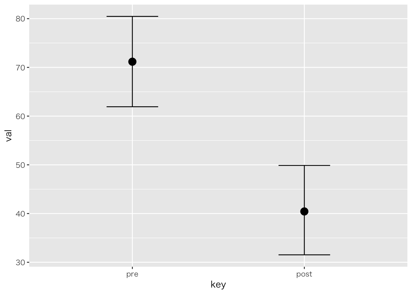

plot(marginal_effects(result.anova3,effects="Text"))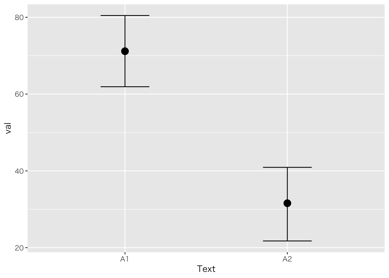

plot(marginal_effects(result.anova3,effects="key:Text"))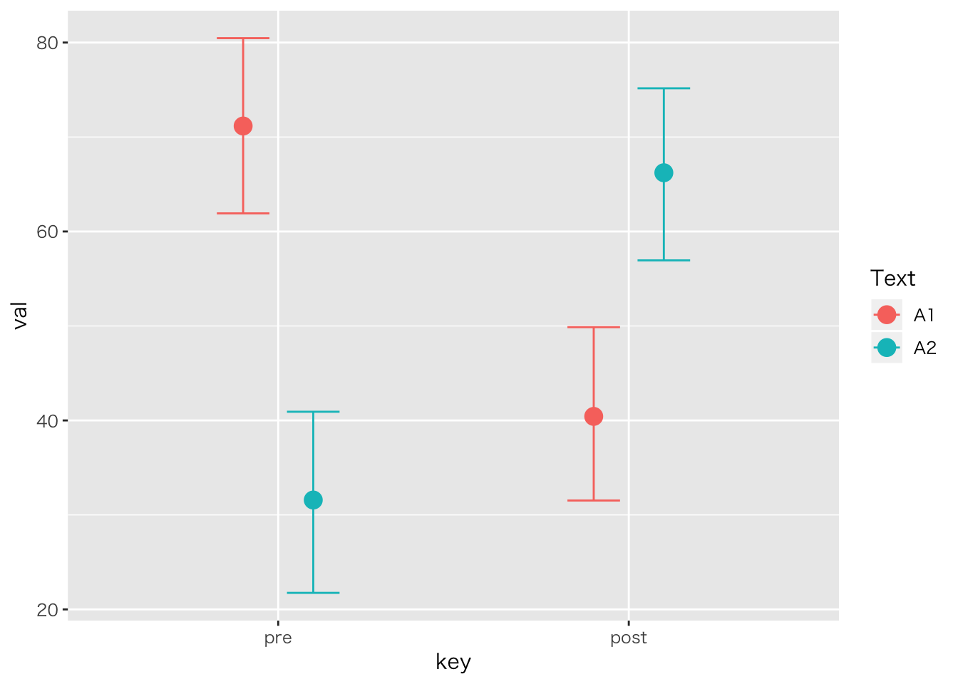

因子分析モデル

こちらからデータをダウンロードしてください(出典；https://www1.doshisha.ac.jp/~mjin/R/Chap_25/25.html)。

library(psych)

## 
## Attaching package: 'psych'

## The following object is masked from 'package:brms':
## 
##     cs

## The following objects are masked from 'package:ggplot2':
## 
##     %+%, alpha

Items <- c("円打点","記号記入","形態照合","名詞比較","図柄照合",
             "平面図判断","計算","語彙","立体図判断","文章完成","算数応用")
FA.dat <- read_csv("CATB50.csv") %>% dplyr::select(-X1) %>% setNames(Items)

## Warning: Missing column names filled in: 'X1' [1]

## Parsed with column specification:
## cols(
##   X1 = col_double(),
##   A = col_double(),
##   B = col_double(),
##   C = col_double(),
##   D = col_double(),
##   E = col_double(),
##   F = col_double(),
##   G = col_double(),
##   H = col_double(),
##   I = col_double(),
##   J = col_double(),
##   K = col_double()
## )

相関行列

cor(FA.dat) %>% print(digits=2)

##            円打点 記号記入 形態照合 名詞比較 図柄照合 平面図判断    計算
## 円打点      1.000    0.387   0.1781    0.046    0.070      0.139  0.0719
## 記号記入    0.387    1.000   0.1476    0.255    0.084      0.274  0.2823
## 形態照合    0.178    0.148   1.0000    0.306    0.424      0.446 -0.0095
## 名詞比較    0.046    0.255   0.3056    1.000    0.479      0.412  0.2328
## 図柄照合    0.070    0.084   0.4235    0.479    1.000      0.397 -0.1914
## 平面図判断  0.139    0.274   0.4456    0.412    0.397      1.000 -0.0539
## 計算        0.072    0.282  -0.0095    0.233   -0.191     -0.054  1.0000
## 語彙        0.050    0.296   0.3017    0.525    0.372      0.323  0.1919
## 立体図判断  0.010    0.223   0.2834    0.409    0.276      0.612  0.0746
## 文章完成   -0.173    0.078   0.2075    0.579    0.413      0.246  0.0545
## 算数応用   -0.147    0.173   0.0470    0.411    0.056      0.265  0.3977
##            語彙 立体図判断 文章完成 算数応用
## 円打点     0.05      0.010   -0.173   -0.147
## 記号記入   0.30      0.223    0.078    0.173
## 形態照合   0.30      0.283    0.207    0.047
## 名詞比較   0.52      0.409    0.579    0.411
## 図柄照合   0.37      0.276    0.413    0.056
## 平面図判断 0.32      0.612    0.246    0.265
## 計算       0.19      0.075    0.055    0.398
## 語彙       1.00      0.233    0.626    0.405
## 立体図判断 0.23      1.000    0.394    0.456
## 文章完成   0.63      0.394    1.000    0.356
## 算数応用   0.41      0.456    0.356    1.000

2-1.screeplot

psych::fa.parallel(FA.dat,fa="fa")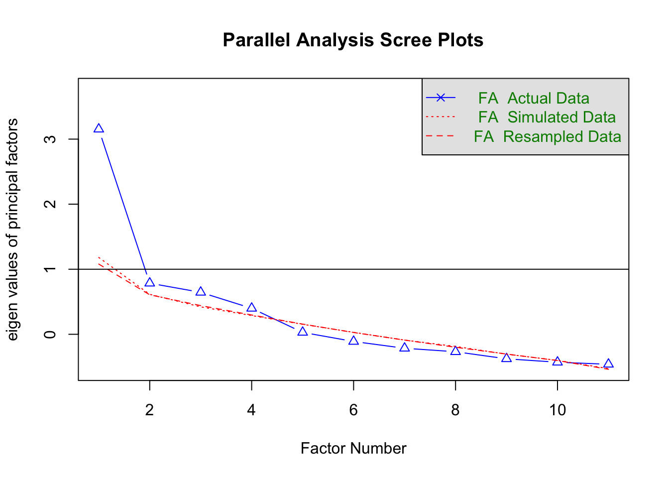

## Parallel analysis suggests that the number of factors =  1  and the number of components =  NA

3.result

fa.result <- fa(FA.dat,4,rotate='none')
print(fa.result,digits=3)

## Factor Analysis using method =  minres
## Call: fa(r = FA.dat, nfactors = 4, rotate = "none")
## Standardized loadings (pattern matrix) based upon correlation matrix
##              MR1    MR2    MR3    MR4    h2    u2  com
## 円打点     0.085 -0.278  0.587  0.201 0.470 0.530 1.74
## 記号記入   0.368  0.034  0.548  0.126 0.453 0.547 1.88
## 形態照合   0.458 -0.342  0.069  0.037 0.333 0.667 1.92
## 名詞比較   0.745  0.075 -0.051  0.144 0.584 0.416 1.10
## 図柄照合   0.559 -0.421 -0.219  0.176 0.569 0.431 2.44
## 平面図判断 0.664 -0.343  0.141 -0.354 0.705 0.295 2.21
## 計算       0.196  0.539  0.350  0.075 0.458 0.542 2.07
## 語彙       0.691  0.140 -0.056  0.338 0.615 0.385 1.56
## 立体図判断 0.653 -0.028  0.035 -0.477 0.656 0.344 1.84
## 文章完成   0.683  0.145 -0.403  0.203 0.692 0.308 1.94
## 算数応用   0.544  0.537  0.012 -0.233 0.638 0.362 2.35
## 
##                         MR1   MR2   MR3   MR4
## SS loadings           3.368 1.117 1.010 0.677
## Proportion Var        0.306 0.102 0.092 0.062
## Cumulative Var        0.306 0.408 0.500 0.561
## Proportion Explained  0.546 0.181 0.164 0.110
## Cumulative Proportion 0.546 0.727 0.890 1.000
## 
## Mean item complexity =  1.9
## Test of the hypothesis that 4 factors are sufficient.
## 
## The degrees of freedom for the null model are  55  and the objective function was  3.895 with Chi Square of  173.329
## The degrees of freedom for the model are 17  and the objective function was  0.275 
## 
## The root mean square of the residuals (RMSR) is  0.028 
## The df corrected root mean square of the residuals is  0.05 
## 
## The harmonic number of observations is  50 with the empirical chi square  4.252  with prob <  0.999 
## The total number of observations was  50  with Likelihood Chi Square =  11.506  with prob <  0.829 
## 
## Tucker Lewis Index of factoring reliability =  1.1647
## RMSEA index =  0  and the 90 % confidence intervals are  0 0.0788
## BIC =  -54.999
## Fit based upon off diagonal values = 0.992
## Measures of factor score adequacy             
##                                                     MR1   MR2   MR3   MR4
## Correlation of (regression) scores with factors   0.948 0.851 0.825 0.807
## Multiple R square of scores with factors          0.899 0.724 0.680 0.651
## Minimum correlation of possible factor scores     0.799 0.447 0.360 0.303

fa.result <- fa(FA.dat,4,rotate='geominQ')

## Loading required namespace: GPArotation

## Warning in fac(r = r, nfactors = nfactors, n.obs = n.obs, rotate =
## rotate, : I am sorry, to do these rotations requires the GPArotation
## package to be installed

print(fa.result,digits=3,cut=0.3)

## Factor Analysis using method =  minres
## Call: fa(r = FA.dat, nfactors = 4, rotate = "geominQ")
## Standardized loadings (pattern matrix) based upon correlation matrix
##              MR1    MR2    MR3    MR4    h2    u2  com
## 円打点                   0.587        0.470 0.530 1.74
## 記号記入   0.368         0.548        0.453 0.547 1.88
## 形態照合   0.458 -0.342               0.333 0.667 1.92
## 名詞比較   0.745                      0.584 0.416 1.10
## 図柄照合   0.559 -0.421               0.569 0.431 2.44
## 平面図判断 0.664 -0.343        -0.354 0.705 0.295 2.21
## 計算              0.539  0.350        0.458 0.542 2.07
## 語彙       0.691                0.338 0.615 0.385 1.56
## 立体図判断 0.653               -0.477 0.656 0.344 1.84
## 文章完成   0.683        -0.403        0.692 0.308 1.94
## 算数応用   0.544  0.537               0.638 0.362 2.35
## 
##                         MR1   MR2   MR3   MR4
## SS loadings           3.368 1.117 1.010 0.677
## Proportion Var        0.306 0.102 0.092 0.062
## Cumulative Var        0.306 0.408 0.500 0.561
## Proportion Explained  0.546 0.181 0.164 0.110
## Cumulative Proportion 0.546 0.727 0.890 1.000
## 
## Mean item complexity =  1.9
## Test of the hypothesis that 4 factors are sufficient.
## 
## The degrees of freedom for the null model are  55  and the objective function was  3.895 with Chi Square of  173.329
## The degrees of freedom for the model are 17  and the objective function was  0.275 
## 
## The root mean square of the residuals (RMSR) is  0.028 
## The df corrected root mean square of the residuals is  0.05 
## 
## The harmonic number of observations is  50 with the empirical chi square  4.252  with prob <  0.999 
## The total number of observations was  50  with Likelihood Chi Square =  11.506  with prob <  0.829 
## 
## Tucker Lewis Index of factoring reliability =  1.1647
## RMSEA index =  0  and the 90 % confidence intervals are  0 0.0788
## BIC =  -54.999
## Fit based upon off diagonal values = 0.992
## Measures of factor score adequacy             
##                                                     MR1   MR2   MR3   MR4
## Correlation of (regression) scores with factors   0.948 0.851 0.825 0.807
## Multiple R square of scores with factors          0.899 0.724 0.680 0.651
## Minimum correlation of possible factor scores     0.799 0.447 0.360 0.303

plot

fa.result$loadings %>% as.matrix() %>% c() %>% matrix(ncol=4) %>% data.frame() %>% 
  rename(FA1=X1,FA2=X2,FA3=X3,FA4=X4)  %>% 
  mutate(items=Items) %>% 
  tidyr::gather(key,val,-items,factor_key=T) %>% 
  ggplot(aes(x=items,y=val,fill=items))+geom_bar(stat='identity')+facet_wrap(~key)+
  theme(axis.text.x = element_text(angle = 45, hjust = 1))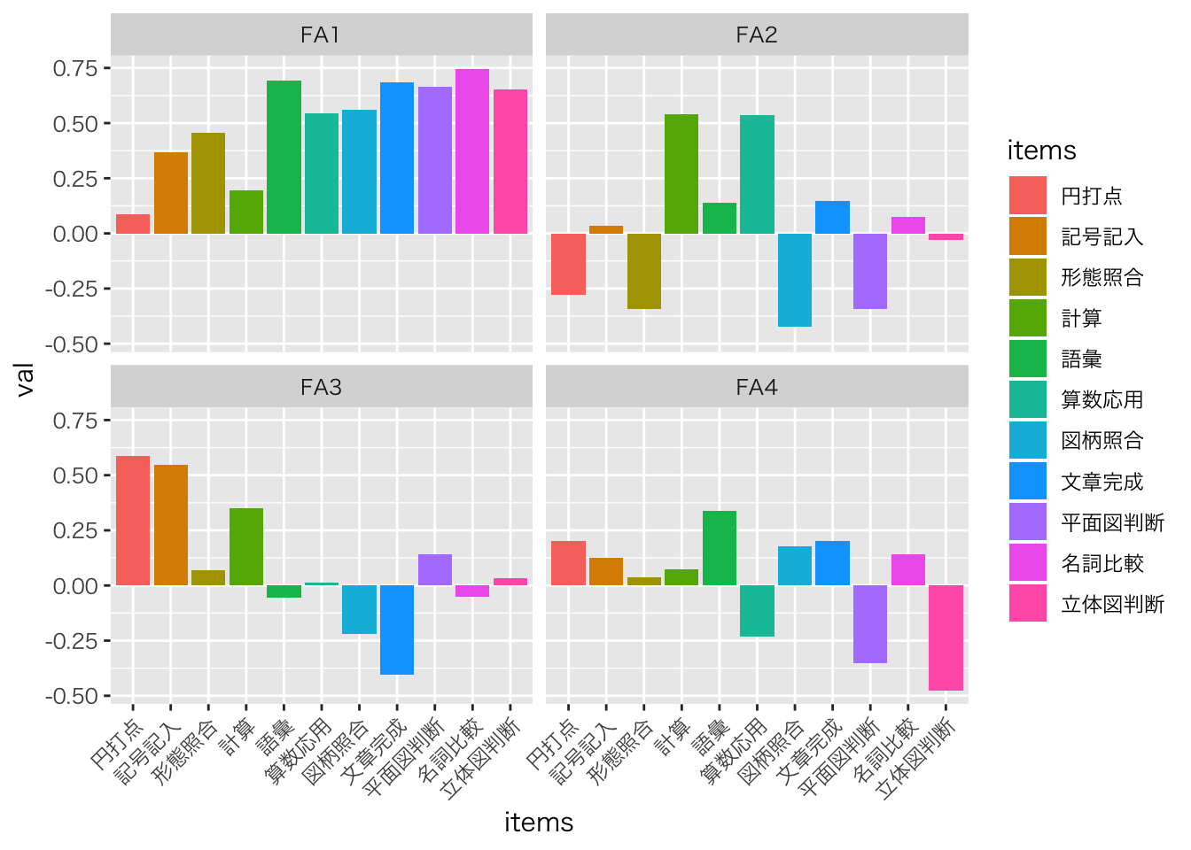

fa.result$scores %>% as.data.frame %>%
  tidyr::gather(key,val,factor_key=TRUE) %>% 
  mutate(因子=factor(key,labels=c("語彙","空間","計算","運動"))) %>% 
  ggplot(aes(x=val,fill=因子))+geom_histogram(binwidth=0.2) + facet_wrap(~因子)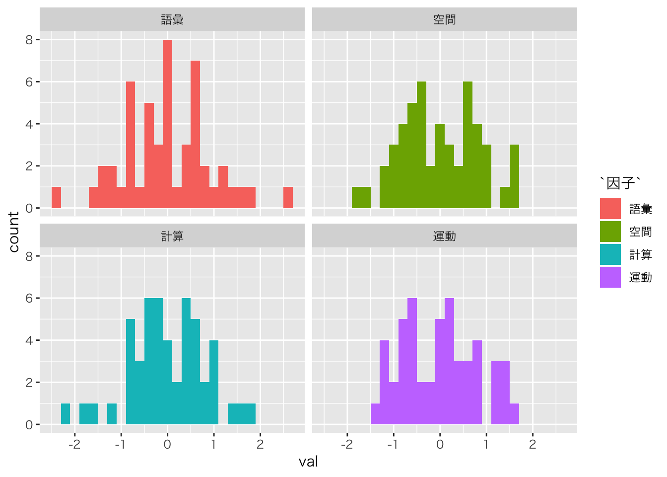

項目反応理論

こちらからデータをダウンロードしてください。

1PL model

library(ltm)

## Loading required package: msm

## Loading required package: polycor

## 
## Attaching package: 'polycor'

## The following object is masked from 'package:psych':
## 
##     polyserial

## 
## Attaching package: 'ltm'

## The following object is masked from 'package:psych':
## 
##     factor.scores

dat <- read_csv("YUtest.csv") %>% 
  dplyr::select(Q4,Q5,Q6,Q7,Q8,Q9,Q10)

## Parsed with column specification:
## cols(
##   .default = col_double()
## )

## See spec(...) for full column specifications.

result.ltm1 <- rasch(dat)
summary(result.ltm1)

## 
## Call:
## rasch(data = dat)
## 
## Model Summary:
##    log.Lik     AIC      BIC
##  -51.61251 119.225 127.1909
## 
## Coefficients:
##              value std.err  z.vals
## Dffclt.Q4  -0.2175  0.3397 -0.6402
## Dffclt.Q5  -0.7099  0.3477 -2.0418
## Dffclt.Q6  -0.8839  0.3623 -2.4398
## Dffclt.Q7  -1.8979  0.6007 -3.1594
## Dffclt.Q8  -1.8980  0.6008 -3.1593
## Dffclt.Q9  -0.7100  0.3477 -2.0420
## Dffclt.Q10 -1.5343  0.4698 -3.2658
## Dscrmn      2.6777  0.9014  2.9706
## 
## Integration:
## method: Gauss-Hermite
## quadrature points: 21 
## 
## Optimization:
## Convergence: 0 
## max(|grad|): 0.00028 
## quasi-Newton: BFGS

plot(result.ltm1,type="ICC",items = c(1,3,5))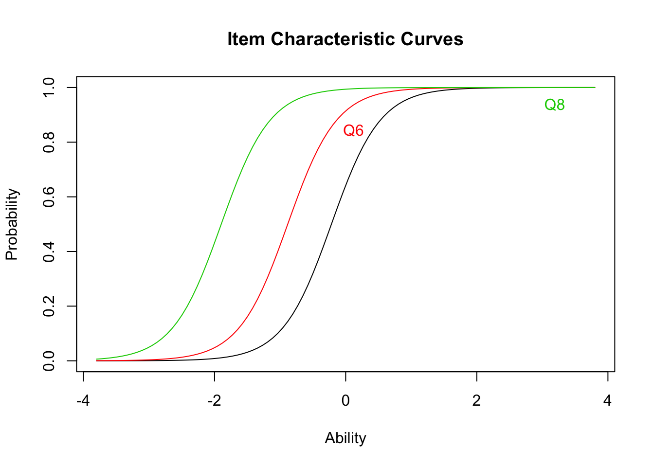

plot(result.ltm1,type="IIC",items = c(1,3,5))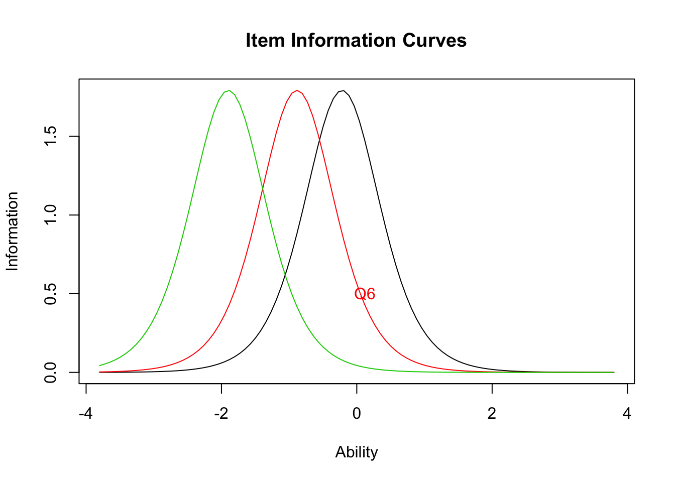

plot(result.ltm1,type="IIC",items = 0)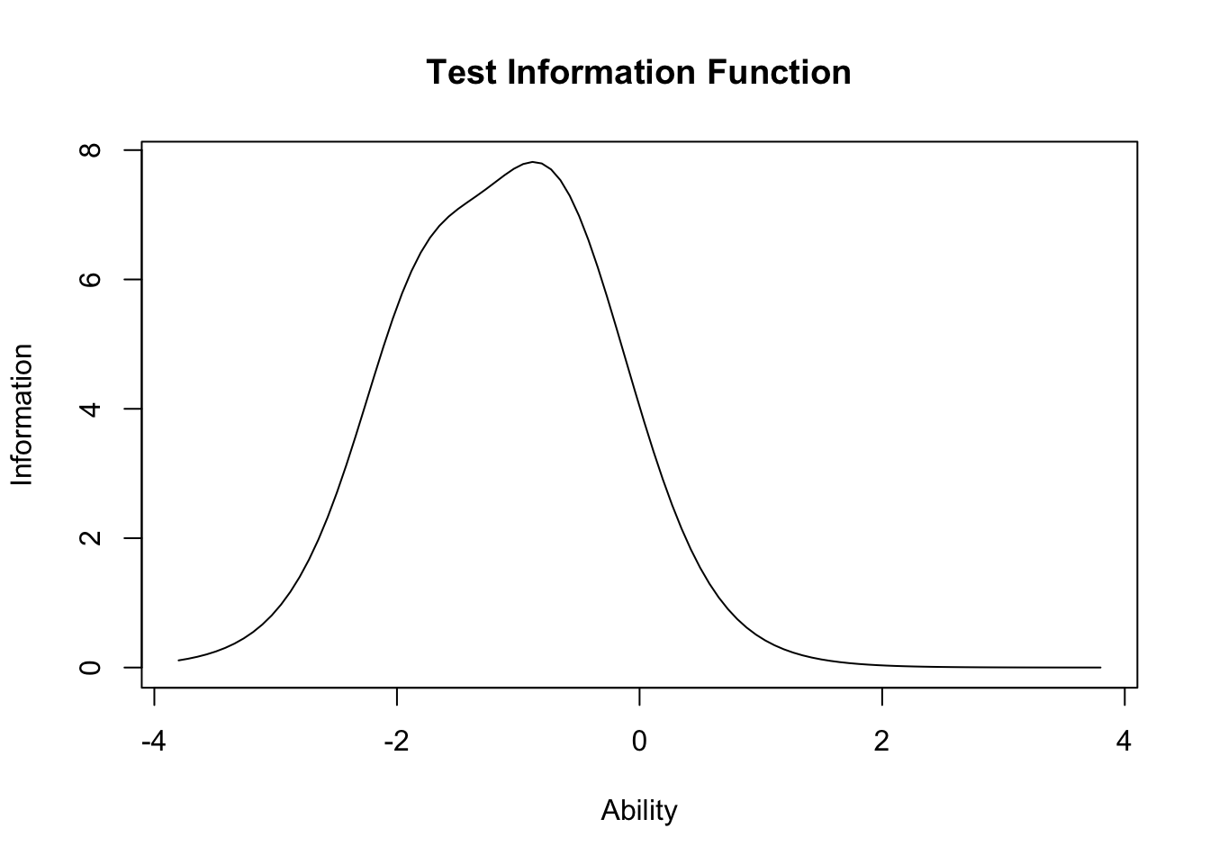

2PL model

result.ltm2 <- ltm(dat~z1)
summary(result.ltm2)

## 
## Call:
## ltm(formula = dat ~ z1)
## 
## Model Summary:
##    log.Lik      AIC      BIC
##  -49.13463 126.2693 140.2095
## 
## Coefficients:
##              value   std.err  z.vals
## Dffclt.Q4  -0.3040    0.2954 -1.0291
## Dffclt.Q5  -0.6871    0.7125 -0.9643
## Dffclt.Q6  -0.8090    0.6888 -1.1746
## Dffclt.Q7  -2.5026    2.2305 -1.1220
## Dffclt.Q8  -8.2500   26.7117 -0.3089
## Dffclt.Q9  -0.7623    0.3072 -2.4812
## Dffclt.Q10 -2.1862    1.4812 -1.4759
## Dscrmn.Q4   3.8676    2.9880  1.2944
## Dscrmn.Q5  22.1274 1736.8954  0.0127
## Dscrmn.Q6   7.5818   41.3155  0.1835
## Dscrmn.Q7   1.6349    2.4491  0.6675
## Dscrmn.Q8   0.3686    1.2518  0.2945
## Dscrmn.Q9   2.8784    1.9777  1.4554
## Dscrmn.Q10  1.3471    1.3926  0.9674
## 
## Integration:
## method: Gauss-Hermite
## quadrature points: 21 
## 
## Optimization:
## Convergence: 0 
## max(|grad|): 0.00011 
## quasi-Newton: BFGS

plot(result.ltm2,type="ICC",items = c(1,3,5))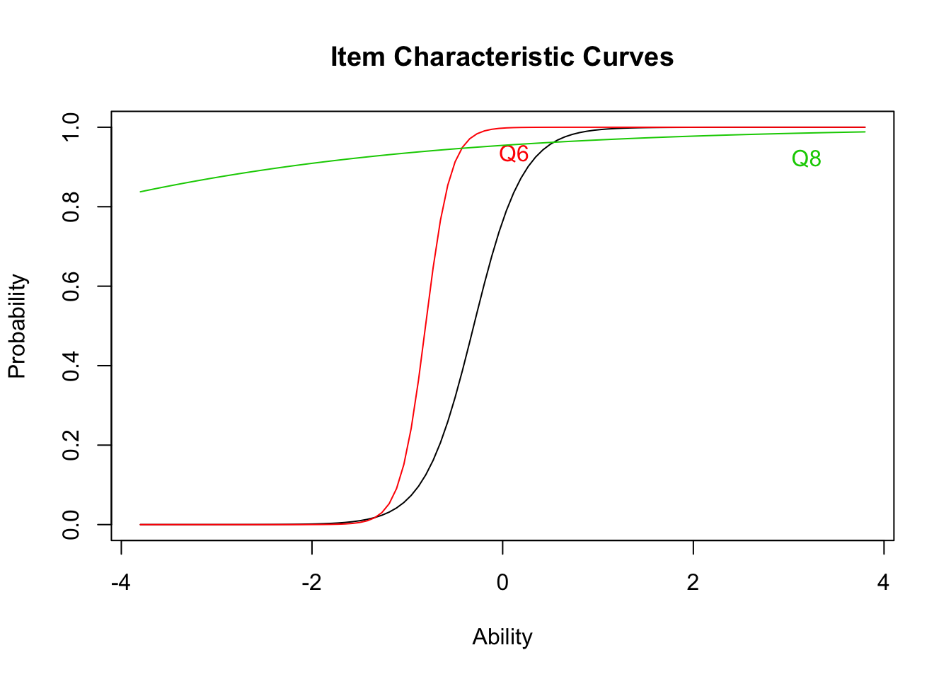

plot(result.ltm2,type="IIC",items = c(1,3,5))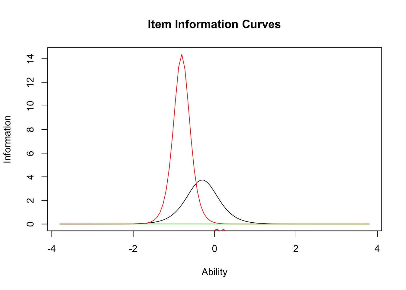

plot(result.ltm2,type="IIC",items = 0)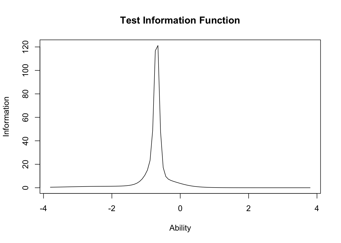

課題7

ここからポケモンのデータ(出典；http://rikapoke.hatenablog.jp/entry/pokemon_datasheet_gne7)をダウンロードし，
次のいずれかの分析をやって遊んでください。
- 様々な能力値の類似性から，MDSかクラスター分析をする
- 様々な能力値がタイプや特性によって違いがあるか線形モデルで分析する
- 様々な能力値を因子分析し，潜在能力がどの程度に分割されるか分析する

pockemon <- read_csv("pokemon_status.csv") %>% 
  dplyr::mutate(ID=row.names(.),
                name=as.factor(ポケモン名),
                type1=as.factor(タイプ１),
                type2=as.factor(タイプ２),
                property1 = as.factor(通常特性１),
                property2 = as.factor(通常特性２),
                propertyD = as.factor(夢特性))

## Parsed with column specification:
## cols(
##   図鑑番号 = col_character(),
##   ポケモン名 = col_character(),
##   タイプ１ = col_character(),
##   タイプ２ = col_character(),
##   通常特性１ = col_character(),
##   通常特性２ = col_character(),
##   夢特性 = col_character(),
##   HP = col_double(),
##   こうげき = col_double(),
##   ぼうぎょ = col_double(),
##   とくこう = col_double(),
##   とくぼう = col_double(),
##   すばやさ = col_double(),
##   合計 = col_double()
## )

summary(pockemon)

##    図鑑番号          ポケモン名          タイプ１        
##  Length:909         Length:909         Length:909        
##  Class :character   Class :character   Class :character  
##  Mode  :character   Mode  :character   Mode  :character  
##                                                          
##                                                          
##                                                          
##                                                          
##    タイプ２          通常特性１         通常特性２       
##  Length:909         Length:909         Length:909        
##  Class :character   Class :character   Class :character  
##  Mode  :character   Mode  :character   Mode  :character  
##                                                          
##                                                          
##                                                          
##                                                          
##     夢特性                HP           こうげき         ぼうぎょ     
##  Length:909         Min.   :  1.0   Min.   :  5.00   Min.   :  5.00  
##  Class :character   1st Qu.: 50.0   1st Qu.: 55.00   1st Qu.: 50.00  
##  Mode  :character   Median : 66.0   Median : 75.00   Median : 70.00  
##                     Mean   : 69.5   Mean   : 79.59   Mean   : 74.24  
##                     3rd Qu.: 80.0   3rd Qu.:100.00   3rd Qu.: 90.00  
##                     Max.   :255.0   Max.   :190.00   Max.   :230.00  
##                                                                      
##     とくこう         とくぼう         すばやさ           合計      
##  Min.   : 10.00   Min.   : 20.00   Min.   :  5.00   Min.   :175.0  
##  1st Qu.: 50.00   1st Qu.: 50.00   1st Qu.: 45.00   1st Qu.:330.0  
##  Median : 65.00   Median : 70.00   Median : 65.00   Median :455.0  
##  Mean   : 72.84   Mean   : 72.23   Mean   : 69.19   Mean   :436.3  
##  3rd Qu.: 95.00   3rd Qu.: 90.00   3rd Qu.: 90.00   3rd Qu.:515.0  
##  Max.   :194.00   Max.   :230.00   Max.   :600.00   Max.   :780.0  
##                                                     NA's   :2      
##       ID                    name          type1            type2    
##  Length:909         アーケオス:  1   みず    :123   ひこう    :109  
##  Class :character   アーケン  :  1   ノーマル:110   じめん    : 39  
##  Mode  :character   アーボ    :  1   くさ    : 83   エスパー  : 36  
##                     アーボック:  1   むし    : 78   どく      : 35  
##                     アーマルド:  1   エスパー: 64   フェアリー: 35  
##                     アイアント:  1   ほのお  : 58   (Other)   :233  
##                     (Other)   :903   (Other) :393   NA's      :422  
##         property1            property2            propertyD  
##  ふゆう      : 40   がんじょう    : 14   ちからずく    : 18  
##  すいすい    : 28   おみとおし    : 13   テレパシー    : 17  
##  するどいめ  : 26   シェルアーマー: 11   ぼうじん      : 17  
##  ようりょくそ: 25   せいしんりょく: 10   きんちょうかん: 16  
##  プレッシャー: 23   テクニシャン  : 10   くだけるよろい: 15  
##  いかく      : 22   (Other)       :400   (Other)       :646  
##  (Other)     :745   NA's          :451   NA's          :180

ID	Text	pre	post
1	A1	78	45
2	A1	76	47
3	A1	72	31
4	A1	61	36
5	A1	69	44
6	A2	24	60
7	A2	44	86
8	A2	29	58
9	A2	24	60
10	A2	37	68

ID	Text	pre	post
1	A1	78	45
2	A1	76	47
3	A1	72	31
4	A1	61	36
5	A1	69	44
6	A2	24	60
7	A2	44	86
8	A2	29	58
9	A2	24	60
10	A2	37	68

ID	Text	pre	post
1	A1	78	45
2	A1	76	47
3	A1	72	31
4	A1	61	36
5	A1	69	44
6	A2	24	60
7	A2	44	86
8	A2	29	58
9	A2	24	60
10	A2	37	68