Creates a ggplot2-based visualization of DAG structures from exametrika Bayesian network models. Supports BNM, LDLRA, LDB, and BINET models. Design based on TDE figures with items as rounded rectangles and fields as diamonds.
Usage
plotGraph_gg(
  data,
  layout = "sugiyama",
  direction = "BT",
  node_size = 12,
  label_size = 4,
  arrow_size = 3,
  title = TRUE,
  colors = NULL,
  show_legend = FALSE,
  legend_position = "right"
)
Arguments
- data
An object of class "exametrika" with model type BNM, LDLRA, LDB, or BINET.
- layout
Character string specifying the layout algorithm. Options include "sugiyama" (default, hierarchical), "fr" (Fruchterman-Reingold), "kk" (Kamada-Kawai), "tree", "stress".
- direction
Character string for hierarchical layout direction. Controls the direction of arrows and node placement in hierarchical layouts. Only applies when
layout = "sugiyama"(default)."BT" (default): Bottom-to-Top. Source nodes at bottom, arrows point upward. Use when representing progression or growth (e.g., learning paths).
"TB": Top-to-Bottom. Source nodes at top, arrows point downward. Traditional hierarchical view (e.g., organizational charts).
"LR": Left-to-Right. Source nodes at left, arrows point right. Good for wide displays or process flows.
"RL": Right-to-Left. Source nodes at right, arrows point left. Alternative horizontal layout.
For other layouts (e.g., "fr", "kk"), this parameter is ignored.
- node_size
Numeric value for node size. Default is 12.
- label_size
Numeric value for label text size inside nodes. Default is 4.
- arrow_size
Numeric value for arrow size. Default is 3.
- title
Logical or character. If
TRUE(default), display an auto-generated title. IfFALSE, no title. If a character string, use it as a custom title. For LDLRA, a single string gets " - Rank N" appended; a character vector of length equal to the number of ranks assigns each element as the title for the corresponding rank.- colors
Character vector. Colors for node types. For BNM/LDLRA: single color for Item nodes. For LDB: single color for Field nodes. For BINET: two colors for Class and Field nodes (positional or named). If
NULL(default), uses the default node type colors (Item=purple, Field=green, Class=blue).- show_legend
Logical. If
TRUE, display the node type legend. Default isFALSE.- legend_position
Character. Position of the legend. One of
"right"(default),"top","bottom","left","none".
Value
A list of ggplot objects. For BNM, a single-element list. For LDLRA/LDB, one plot per rank/class. For BINET, the integrated graph.
Details
Design follows TDE figure specifications:
BNM: Items shown as purple circles with numbers inside
LDLRA: Items as circles per rank/class, one plot per rank. Isolated nodes auto-removed
LDB: Fields shown as green diamonds, one plot per rank. Isolated nodes auto-removed
BINET: Integrated graph with Class nodes (blue squares) and Field nodes (green diamonds) as intermediates. Field nodes are smaller and placed between the Class nodes they connect
Direction Guidelines:
Choose the direction that best represents your data structure:
Use BT (default) for learning progression, skill development, or upward growth
Use TB for traditional hierarchies or causal flows
Use LR/RL for temporal sequences or wide-format displays
Auto-Scaling:
The function automatically scales node and arrow sizes based on graph complexity:
1-5 nodes: 100\
6-10 nodes: 80\
11-20 nodes: 60\
21+ nodes: 50\
Arrows maintain a minimum size of 2mm to ensure visibility.
Note
The linetype common option is not applicable to DAG visualization,
as edges are drawn as directed arrows rather than standard lines.
Examples
library(exametrika)
library(ggExametrika)
# BNM example
DAG <- matrix(c(
"Item01", "Item02", "Item02", "Item03",
"Item02", "Item04", "Item03", "Item05",
"Item04", "Item05"
), ncol = 2, byrow = TRUE)
g <- igraph::graph_from_data_frame(DAG)
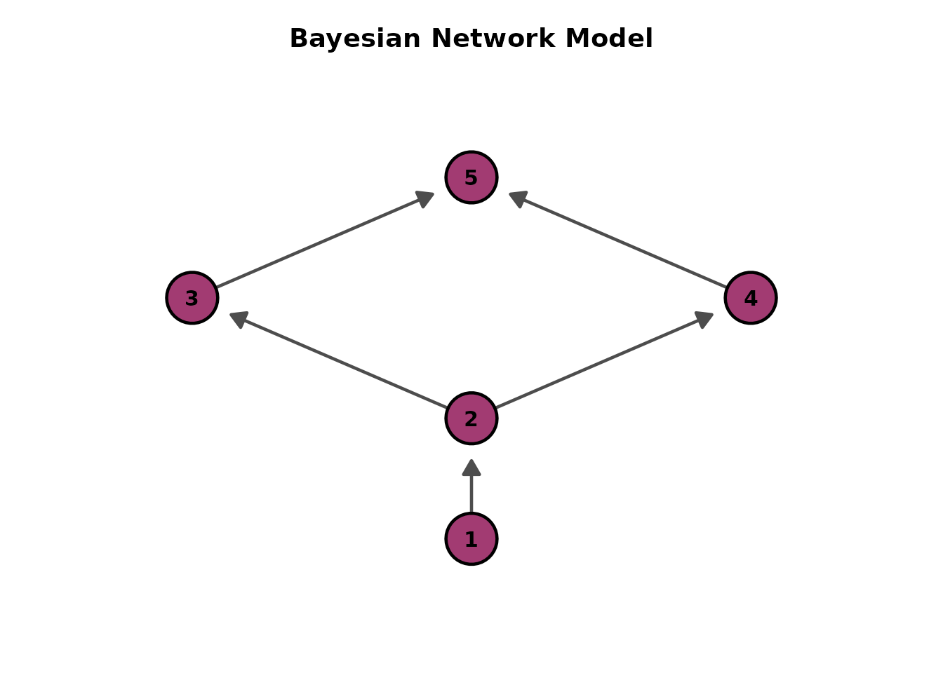
result <- BNM(J5S10, g = g)
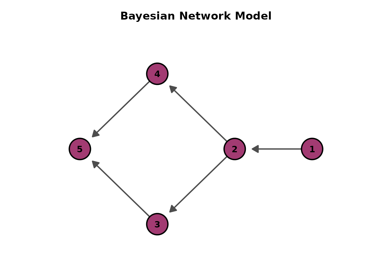
# Default: Bottom-to-Top (arrows point upward)
plots <- plotGraph_gg(result)
plots[[1]]
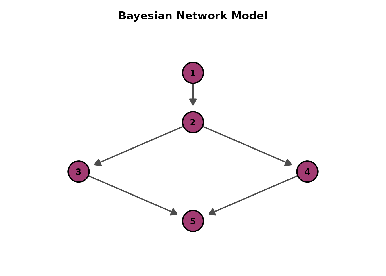
 # Alternative directions
plotGraph_gg(result, direction = "TB")[[1]] # Top-to-Bottom
# Alternative directions
plotGraph_gg(result, direction = "TB")[[1]] # Top-to-Bottom
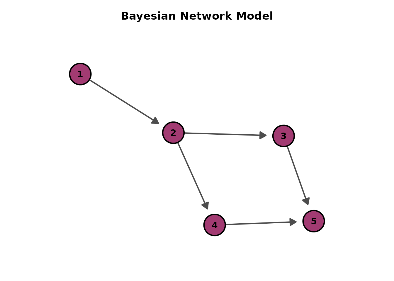
 plotGraph_gg(result, direction = "LR")[[1]] # Left-to-Right
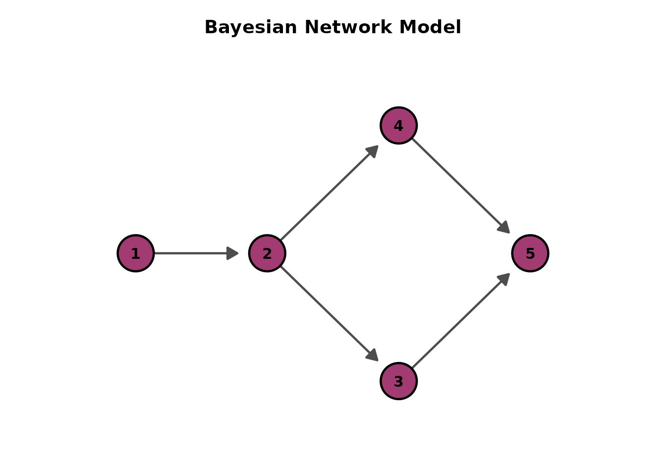 plotGraph_gg(result, direction = "RL")[[1]] # Right-to-Left
 # Force-directed layout (no direction parameter)
plotGraph_gg(result, layout = "fr")[[1]]
# Force-directed layout (no direction parameter)
plotGraph_gg(result, layout = "fr")[[1]]
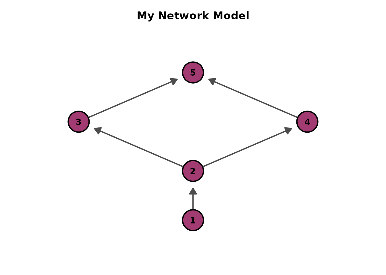
 # Custom title
plotGraph_gg(result, title = "My Network Model")[[1]]
# Custom title
plotGraph_gg(result, title = "My Network Model")[[1]]