Getting Started with ggExametrika
Source:vignettes/articles/getting-started.Rmd
getting-started.RmdOverview
ggExametrika provides ggplot2-based visualization functions for outputs from the exametrika package. It covers a wide range of psychometric models including IRT, GRM, Latent Class/Rank Analysis, Biclustering, Bayesian Network Models, and more.
Setup
library(exametrika)
library(ggExametrika)
#> Loading required package: ggplot2
#>
#> Attaching package: 'ggExametrika'
#> The following objects are masked from 'package:exametrika':
#>
#>     ItemInformationFunc, LogisticModel
1. IRT (Item Response Theory)
IRT models (2PL, 3PL, 4PL) estimate item parameters for binary response data.
result_irt <- IRT(J15S500, model = 2)plotICC_gg: Item Characteristic Curve
Shows the probability of a correct response as a function of ability (theta).
# Returns a list of plots (one per item)
icc_plots <- plotICC_gg(result_irt)
icc_plots[[1]] # Show first item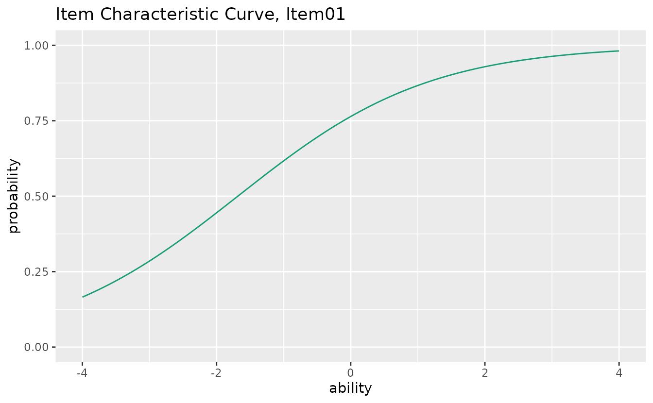
Use combinePlots_gg() to display multiple items at
once:
combinePlots_gg(icc_plots, selectPlots = 1:6)
You can customize the ability range:
icc_plots <- plotICC_gg(result_irt, xvariable = c(-3, 3))plotIIC_gg: Item Information Curve
Displays how precisely each item measures ability at different theta levels.
iic_plots <- plotIIC_gg(result_irt)
iic_plots[[1]]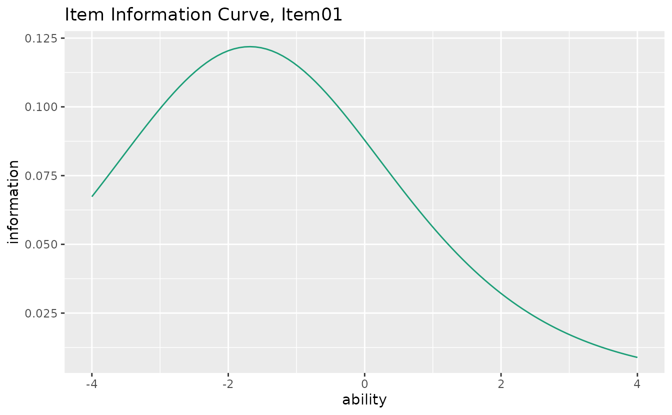
combinePlots_gg(iic_plots, selectPlots = 1:6)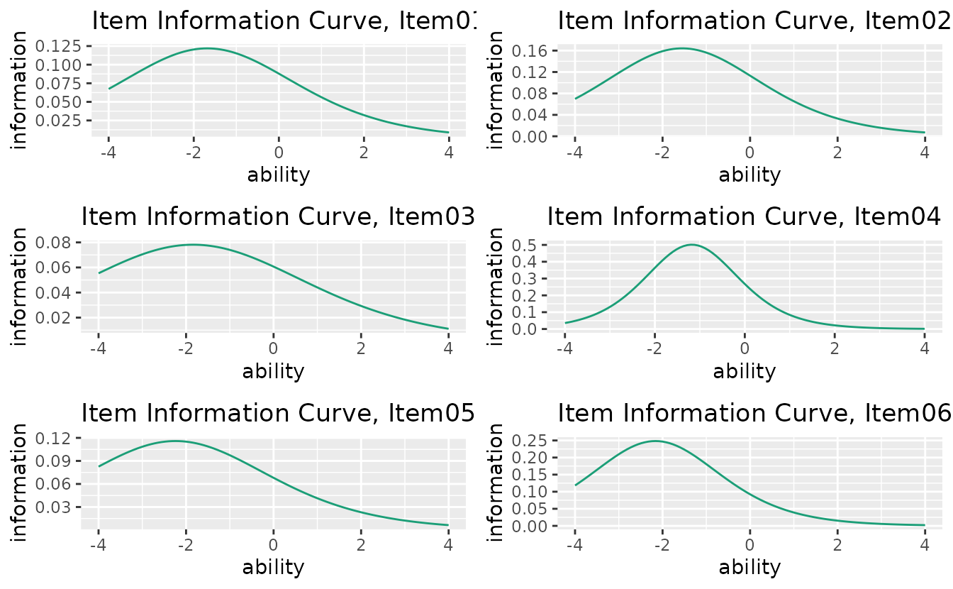
Select specific items:
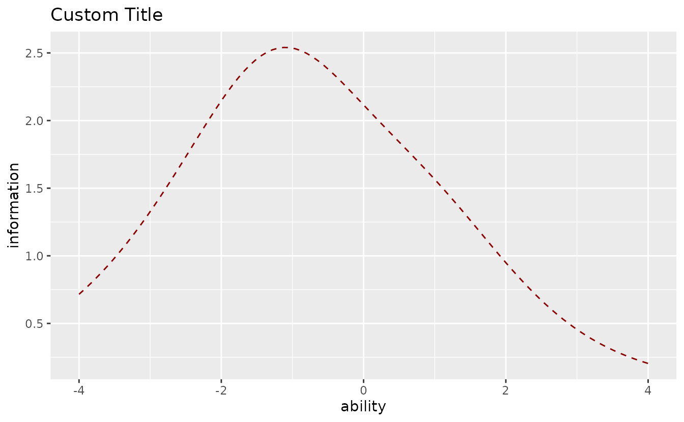
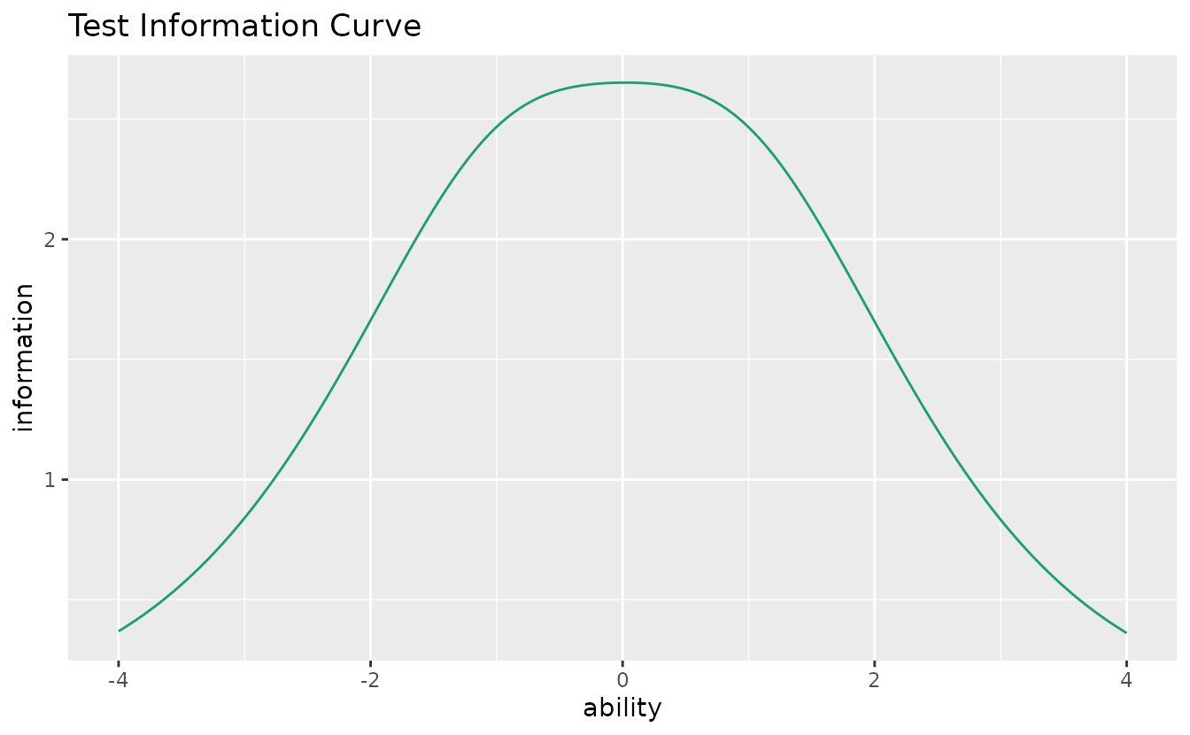
iic_plots <- plotIIC_gg(result_irt, items = c(1, 3, 5))plotTIC_gg: Test Information Curve
Shows the total test information (sum of all item information functions).
tic_plot <- plotTIC_gg(result_irt)
tic_plot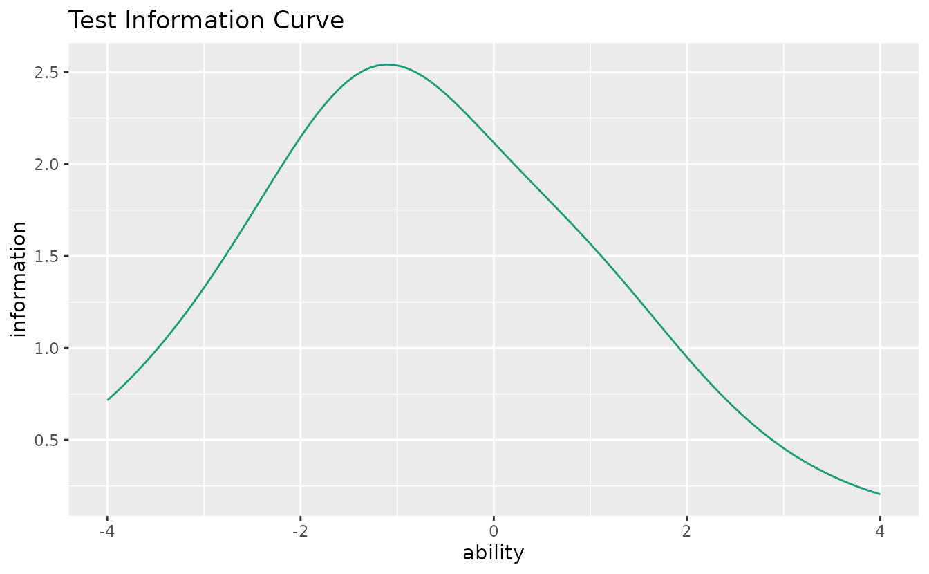
Customize appearance:
plotTIC_gg(result_irt,
  title = "Custom Title",
  colors = "darkred",
  linetype = "dashed"
)
plotTRF_gg: Test Response Function
Shows the expected total score as a function of ability.
trf_plot <- plotTRF_gg(result_irt)
trf_plot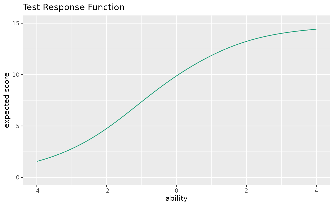
plotICC_overlay_gg: ICC Overlay
Overlays all Item Characteristic Curves on a single plot for easy comparison.
plotICC_overlay_gg(result_irt)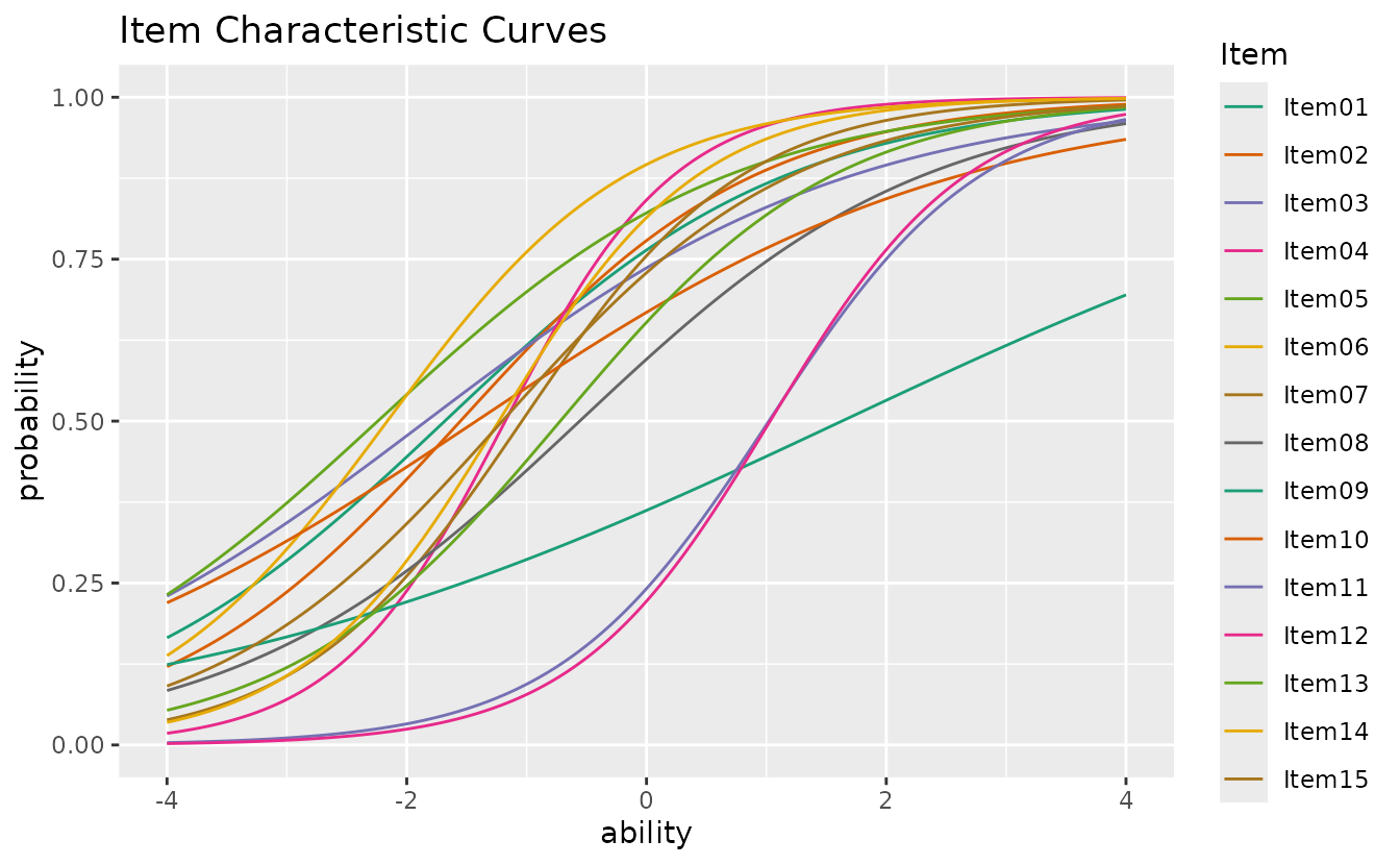
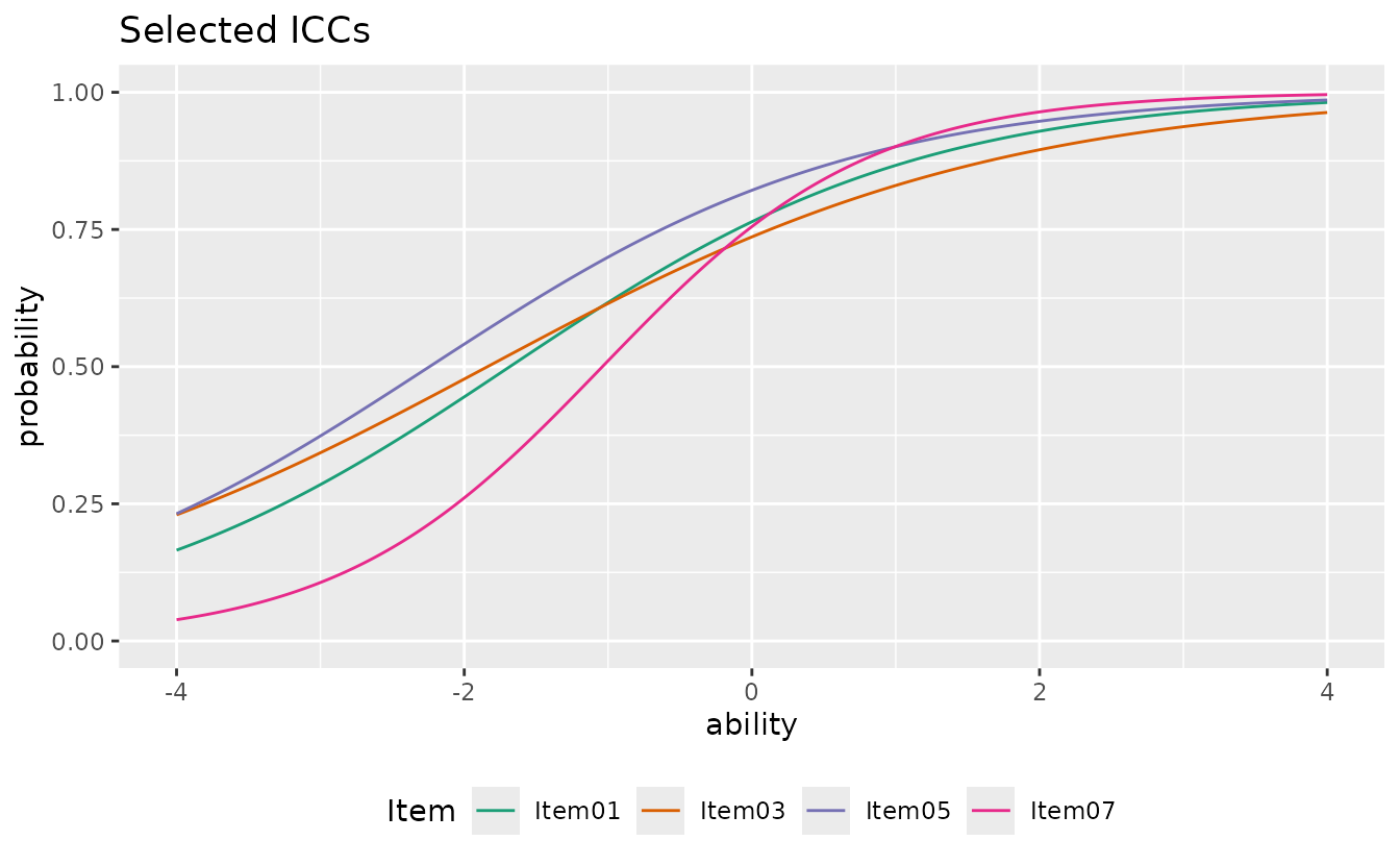
Select specific items and customize:
plotICC_overlay_gg(result_irt,
  items = c(1, 3, 5, 7),
  title = "Selected ICCs",
  linetype = "solid",
  legend_position = "bottom"
)
plotIIC_overlay_gg: IIC Overlay
Overlays all Item Information Curves on a single plot.
plotIIC_overlay_gg(result_irt)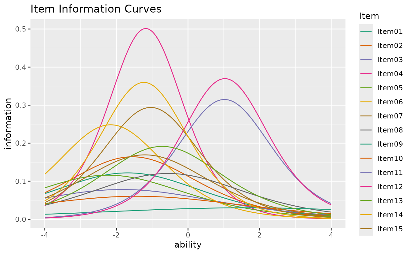
This function also works with GRM (see Section 2).
LogisticModel / ItemInformationFunc: Helper Functions
Low-level computation functions for IRT models.
# 4-parameter logistic model: P(theta)
LogisticModel(x = 0, a = 1.5, b = 0.5, c = 0.2, d = 1.0)
#> [1] 0.456657

# Item information at a given theta
ItemInformationFunc(x = 0, a = 1.5, b = 0.5, c = 0.2, d = 1.0)
#> [1] 0.2755452
2. GRM (Graded Response Model)
GRM handles ordered polytomous response data (e.g., Likert scales).
result_grm <- GRM(J5S1000)plotICRF_gg: Item Category Response Function
Displays the probability of each response category as a function of ability.
icrf_plots <- plotICRF_gg(result_grm)
icrf_plots[[1]]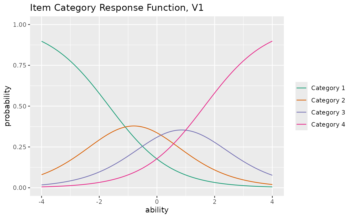
combinePlots_gg(icrf_plots, selectPlots = 1:5)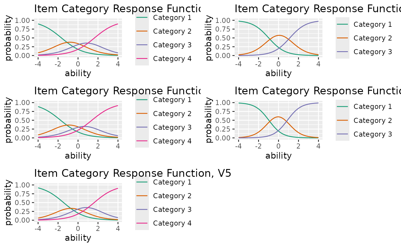
Select specific items and customize:
plotICRF_gg(result_grm,
  items = c(1, 2),
  title = "ICRF for Items 1-2",
  colors = c("#E41A1C", "#377EB8", "#4DAF4A", "#984EA3", "#FF7F00"),
  linetype = "solid",
  show_legend = TRUE,
  legend_position = "bottom"
)
#> [[1]]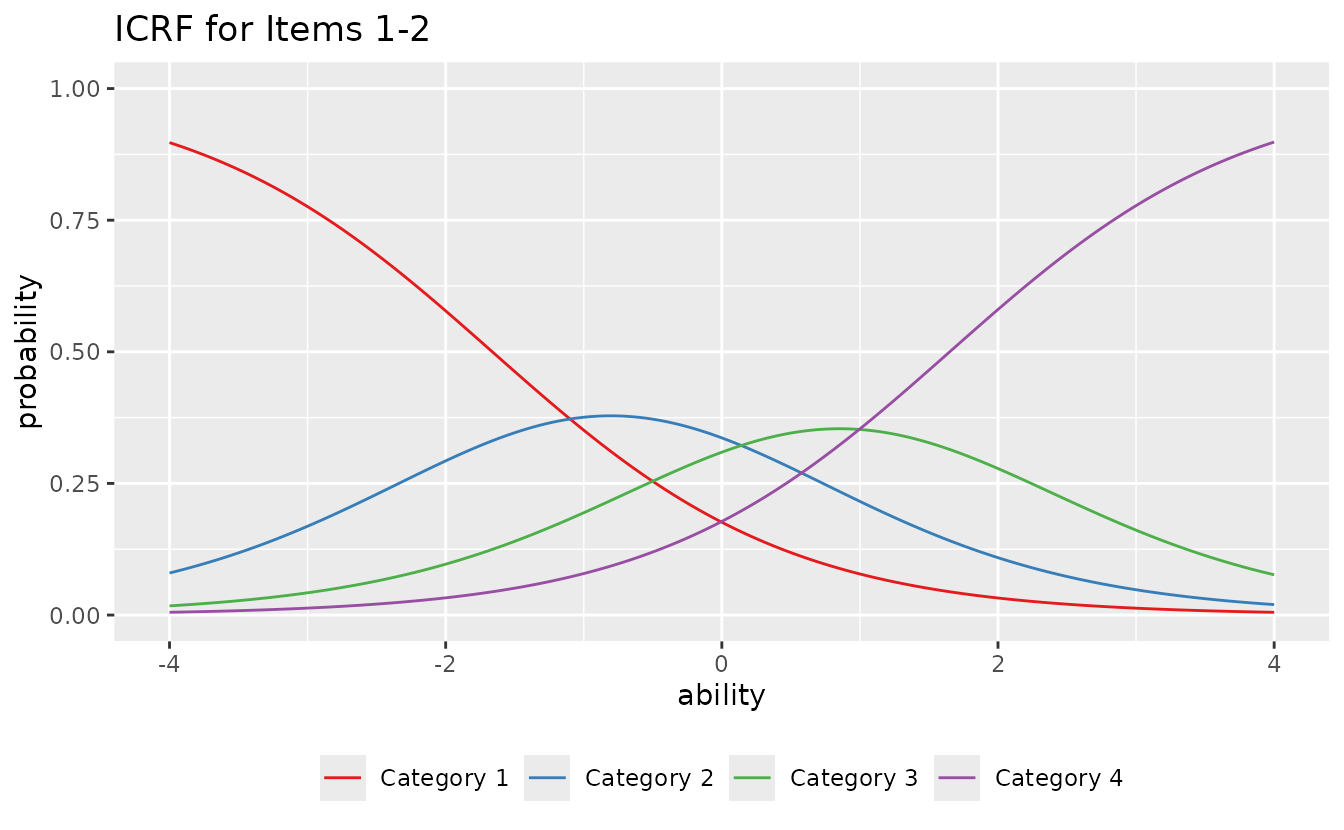
#>
#> [[2]]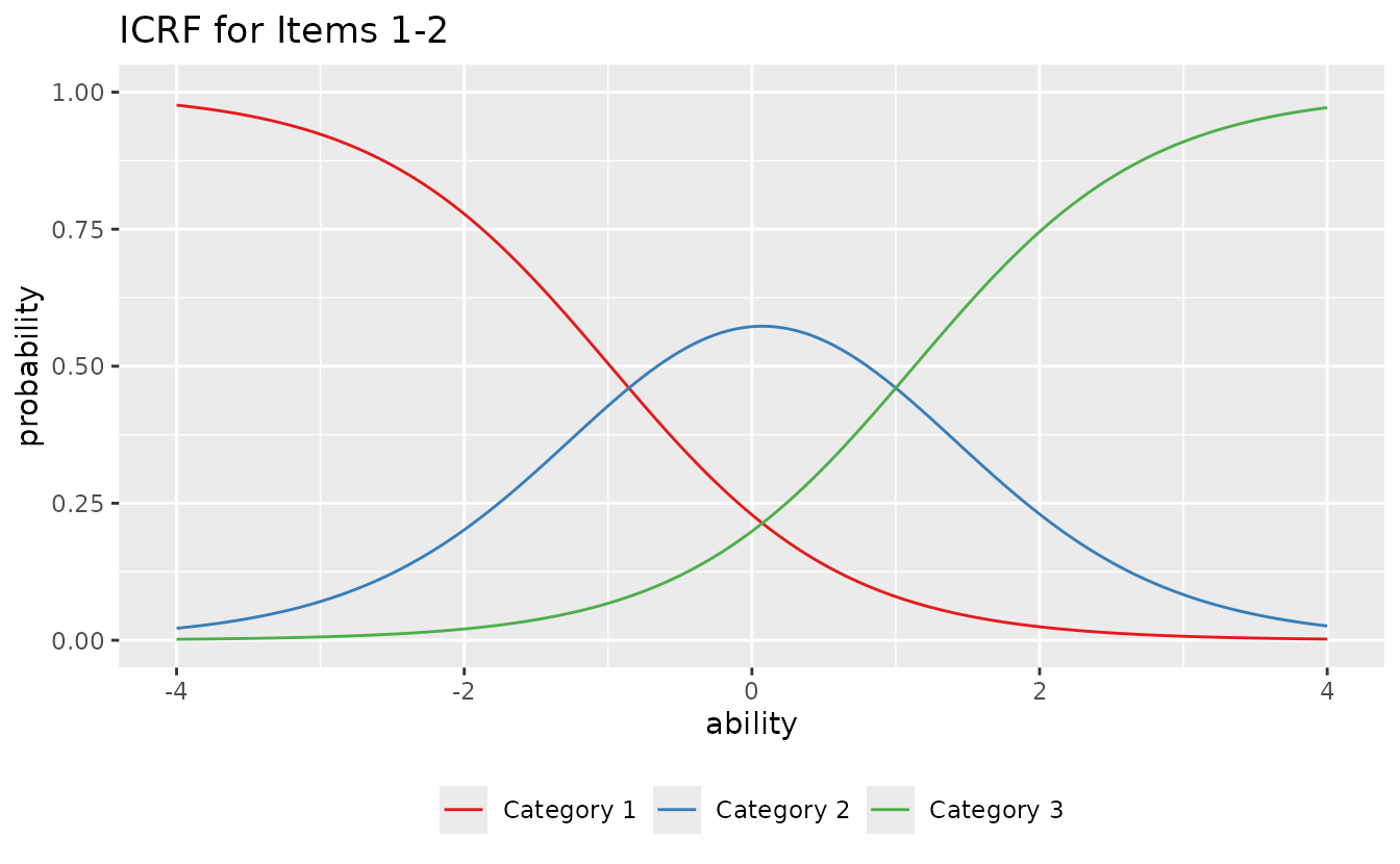
plotIIC_gg (GRM): Item Information Curve
Also works with GRM data:
iic_grm <- plotIIC_gg(result_grm)
iic_grm[[1]]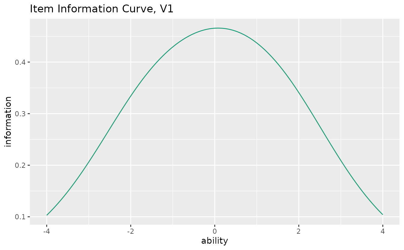
combinePlots_gg(iic_grm, selectPlots = 1:5)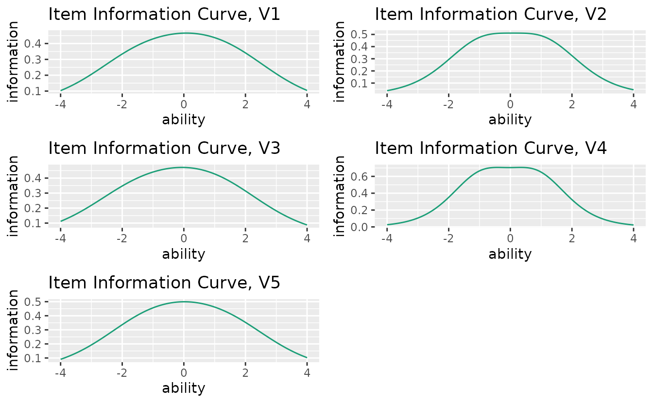
ItemInformationFunc_GRM: Helper Function
# Information at theta = 0 for a 5-category item
ItemInformationFunc_GRM(theta = 0, a = 1.5, b = c(-1.5, -0.5, 0.5, 1.5))
#> [1] 1.368688
3. LCA (Latent Class Analysis)
LCA identifies latent classes (discrete groups) from binary response data.
result_lca <- LCA(J15S500, ncls = 3)plotIRP_gg: Item Reference Profile
Shows the probability of a correct response for each item within each latent class.
irp_plots <- plotIRP_gg(result_lca)
irp_plots[[1]]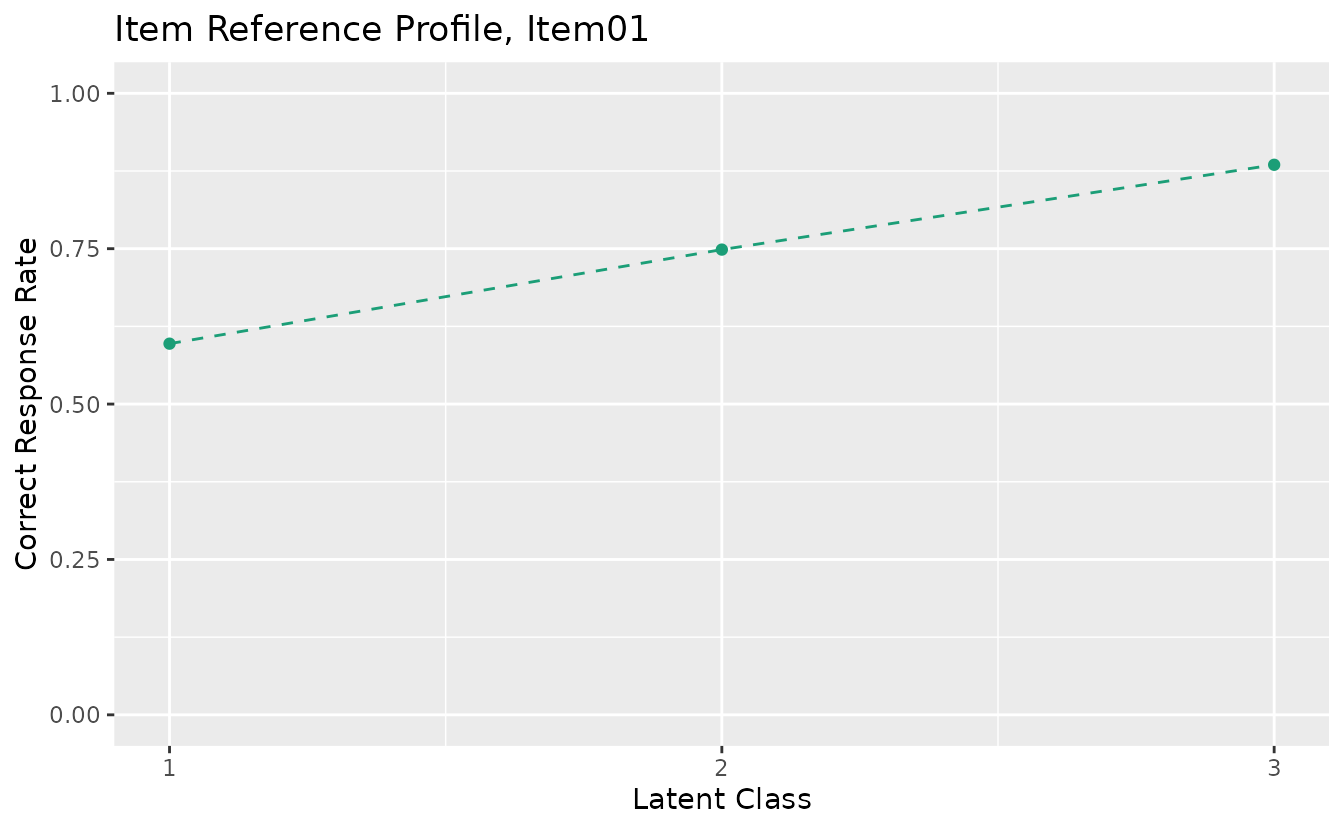
combinePlots_gg(irp_plots, selectPlots = 1:6)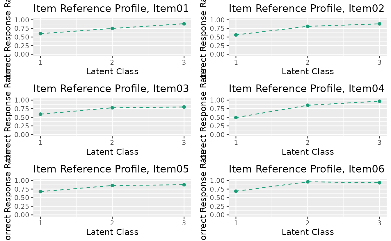
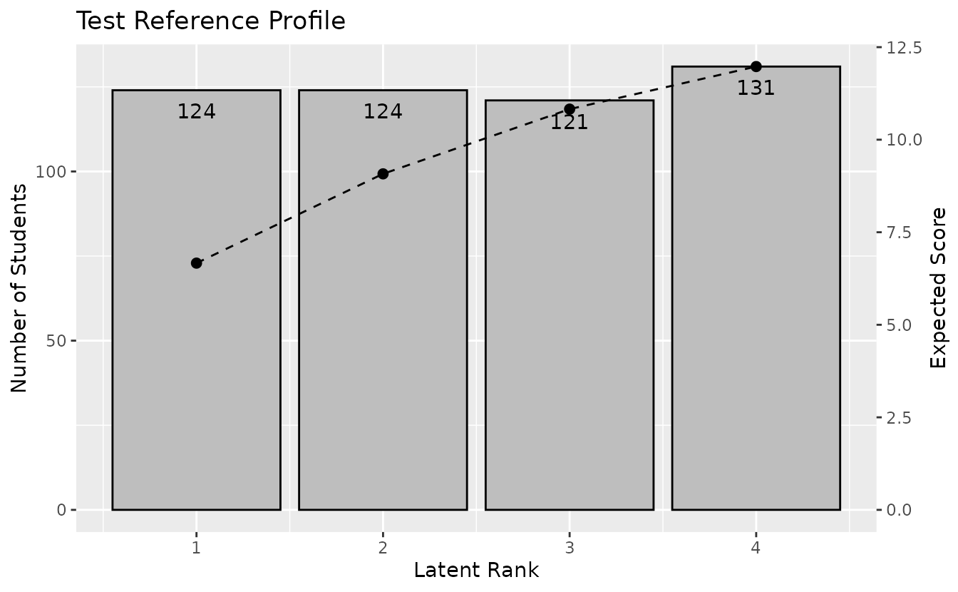
plotTRP_gg: Test Reference Profile
Displays the number of students and expected test score per class.
trp_plot <- plotTRP_gg(result_lca)
trp_plot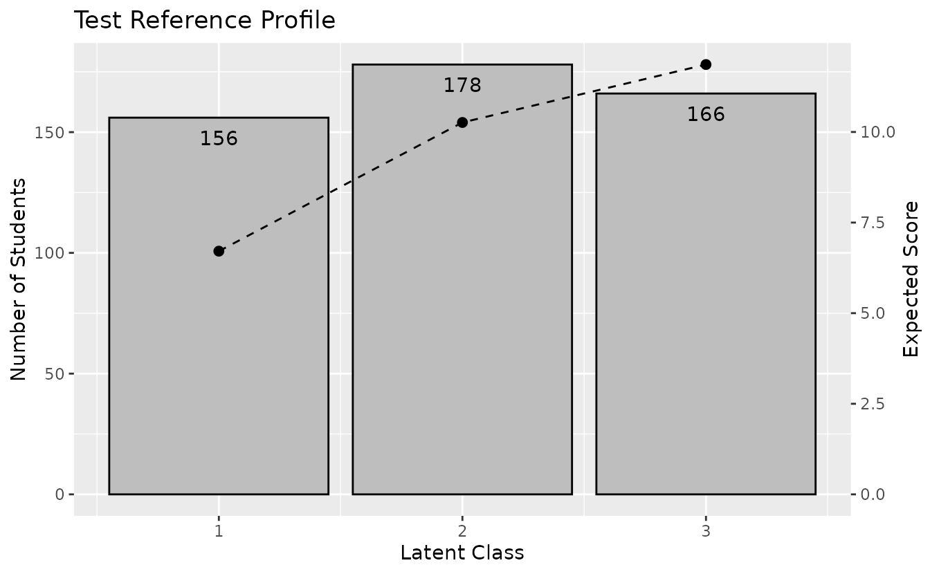
Hide student count labels or title:
plotTRP_gg(result_lca, Num_Students = FALSE, title = FALSE)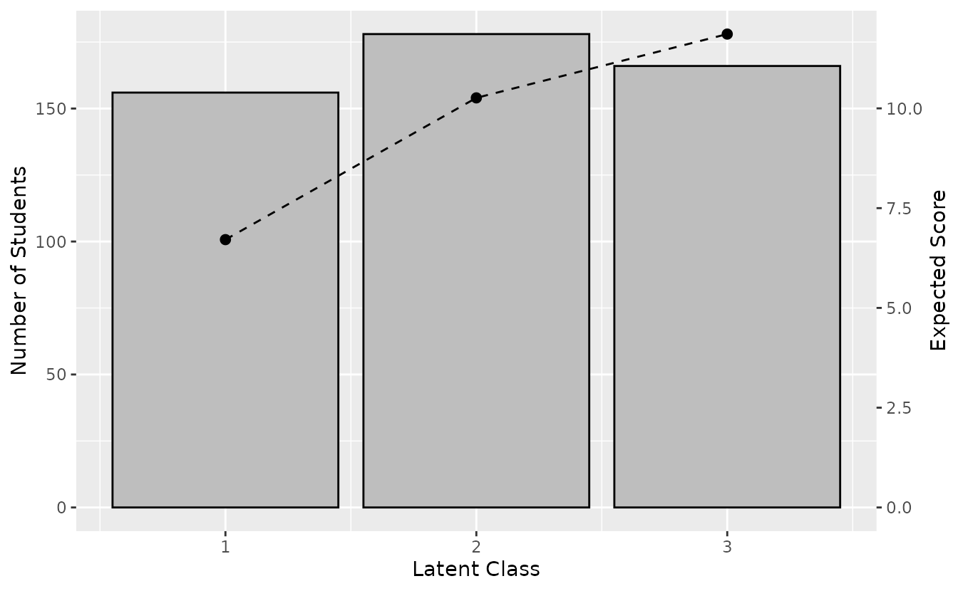
plotLCD_gg: Latent Class Distribution
Displays the class membership distribution.
lcd_plot <- plotLCD_gg(result_lca)
lcd_plot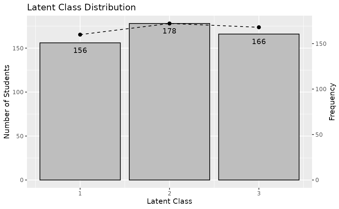
plotCMP_gg: Class Membership Profile
Shows the membership probability profile for each student across all classes.
# Returns a list of plots (one per student)
cmp_plots <- plotCMP_gg(result_lca)
cmp_plots[[1]] # First student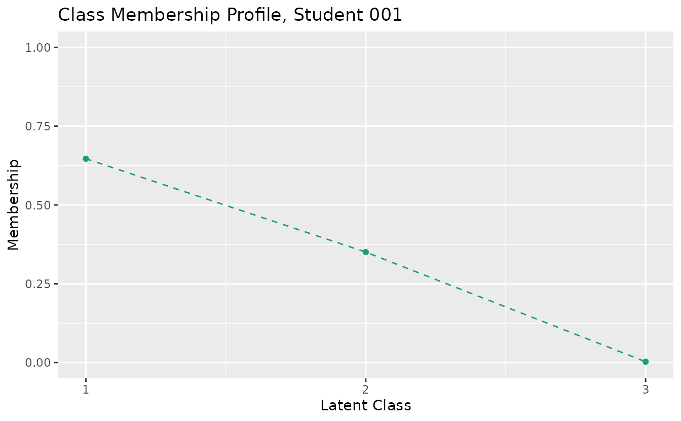
combinePlots_gg(cmp_plots, selectPlots = 1:6)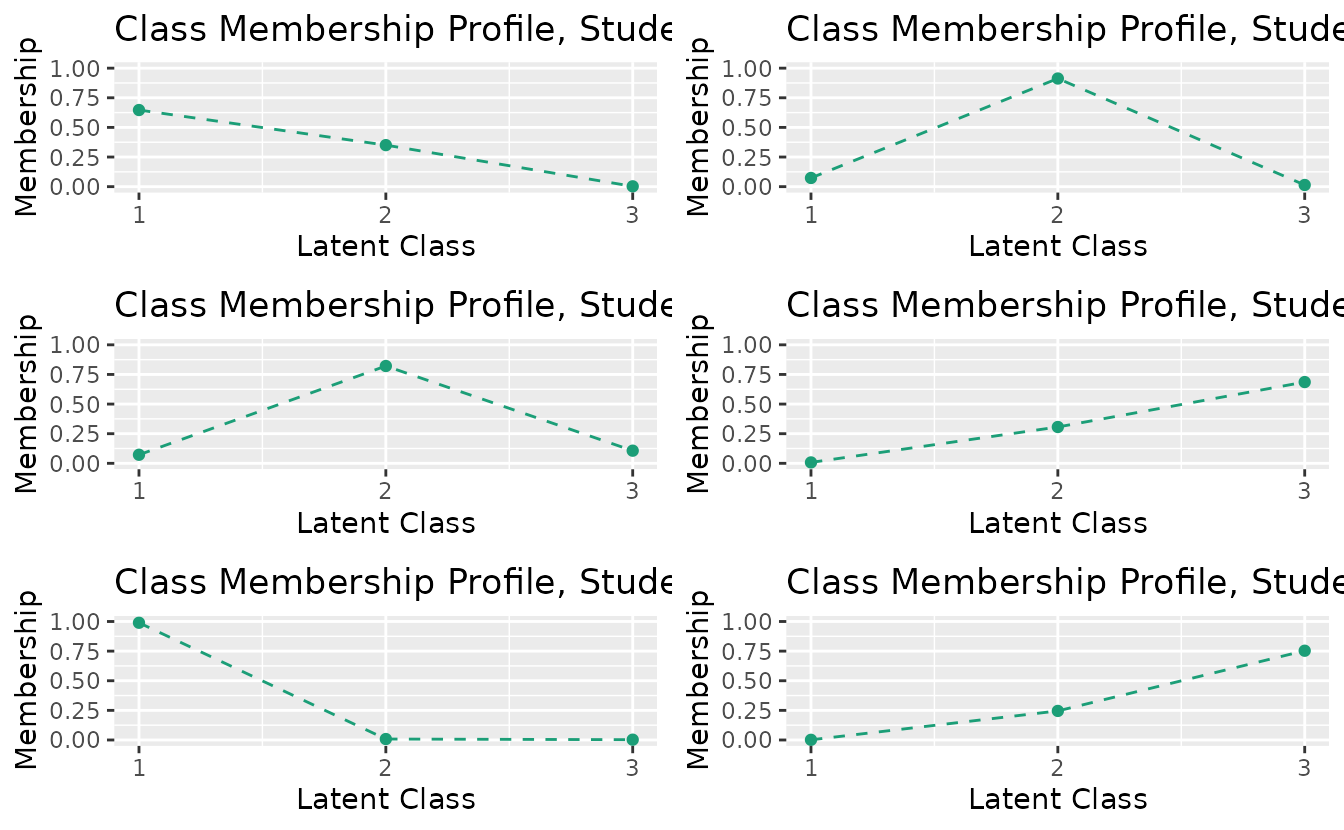
4. LRA (Latent Rank Analysis)
LRA identifies ordered latent ranks from binary response data.
result_lra <- LRA(J15S500, nrank = 4)plotIRP_gg: Item Reference Profile
irp_plots <- plotIRP_gg(result_lra)
combinePlots_gg(irp_plots, selectPlots = 1:6)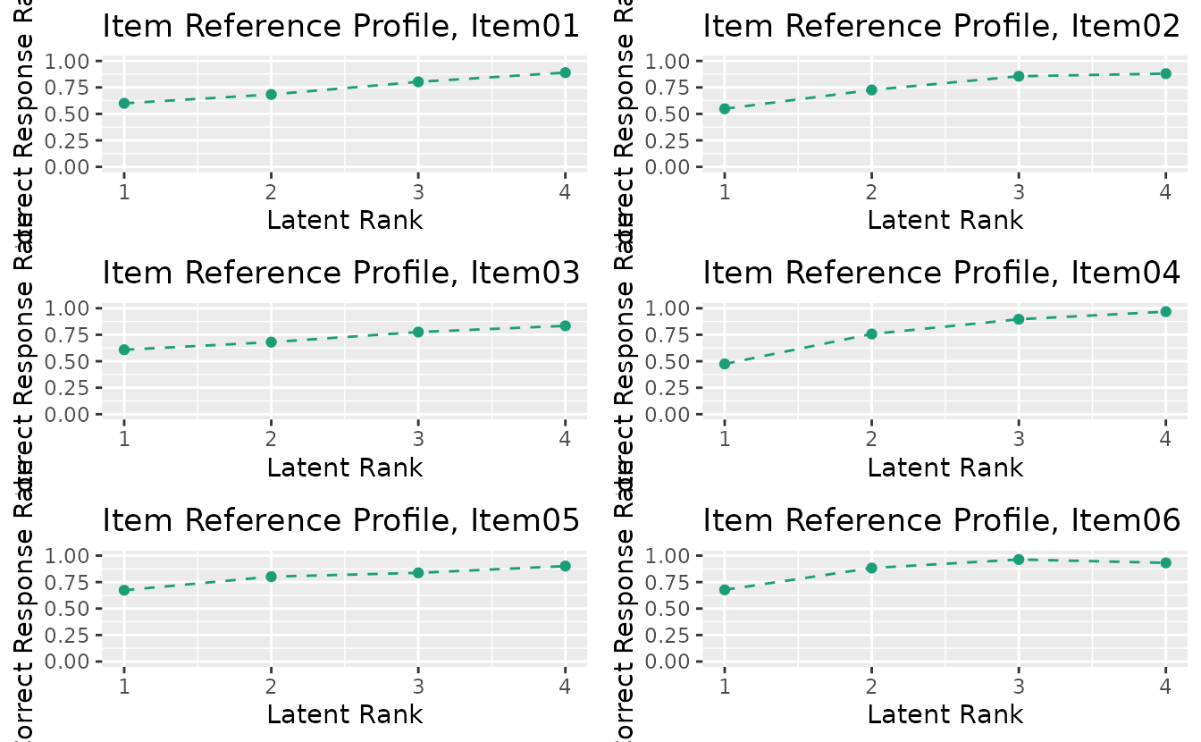
plotLRD_gg: Latent Rank Distribution
Displays the rank membership distribution.
lrd_plot <- plotLRD_gg(result_lra)
lrd_plot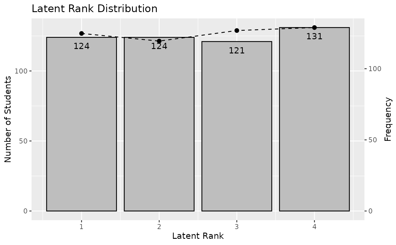
plotRMP_gg: Rank Membership Profile
Shows the membership probability profile for each student across all ranks.
rmp_plots <- plotRMP_gg(result_lra)
rmp_plots[[1]]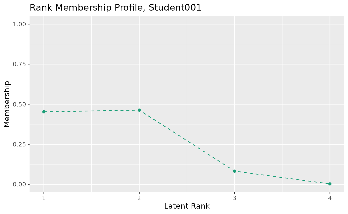
combinePlots_gg(rmp_plots, selectPlots = 1:6)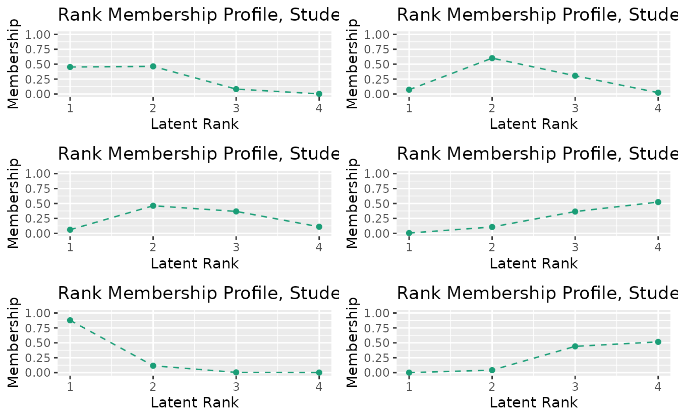
4b. LRAordinal / LRArated (Polytomous Latent Rank Analysis)
LRAordinal and LRArated handle ordinal and rated polytomous response data, providing specialized visualizations for score distributions and category-level analysis.
result_lra_ord <- LRA(J15S3810, nrank = 4, dataType = "ordinal")plotScoreFreq_gg: Score Frequency Distribution
Shows the density distribution of scores with vertical lines indicating rank boundary thresholds.
plotScoreFreq_gg(result_lra_ord)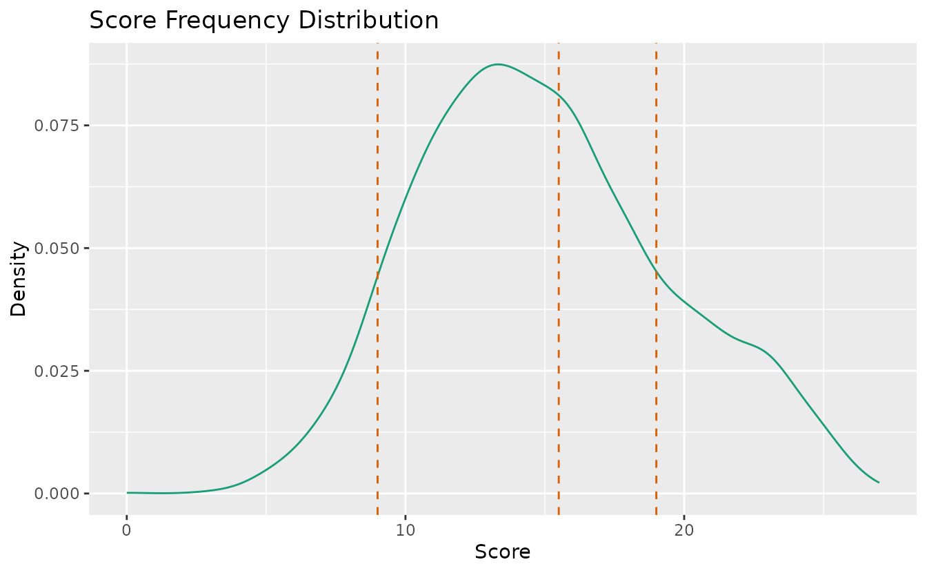
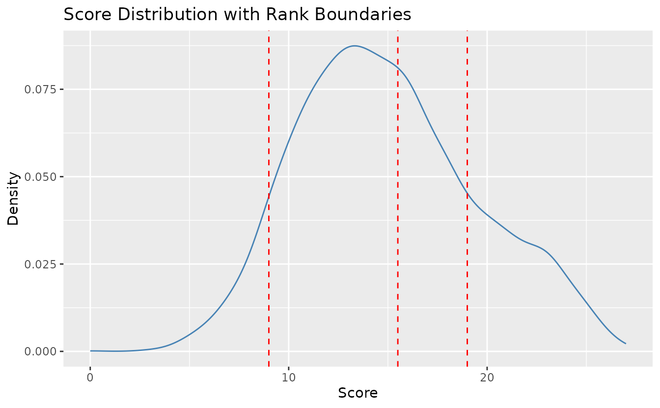
Customize colors and line types:
plotScoreFreq_gg(result_lra_ord,
  title = "Score Distribution with Rank Boundaries",
  colors = c("steelblue", "red"),
  linetype = c("solid", "dashed")
)
plotScoreRank_gg: Score-Rank Heatmap
Displays the joint distribution of observed scores and estimated ranks as a heatmap. Darker cells indicate higher frequency.
plotScoreRank_gg(result_lra_ord)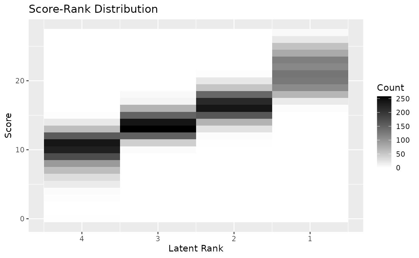
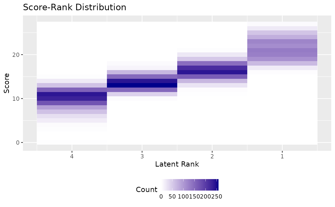
Customize gradient colors:
plotScoreRank_gg(result_lra_ord,
  title = "Score-Rank Distribution",
  colors = c("white", "darkblue"),
  legend_position = "bottom"
)
plotICRP_gg: Item Category Reference Profile
Shows the probability of selecting each response category across latent ranks. Probabilities at each rank sum to 1.0.
icrp_plots <- plotICRP_gg(result_lra_ord, items = 1:4)
icrp_plots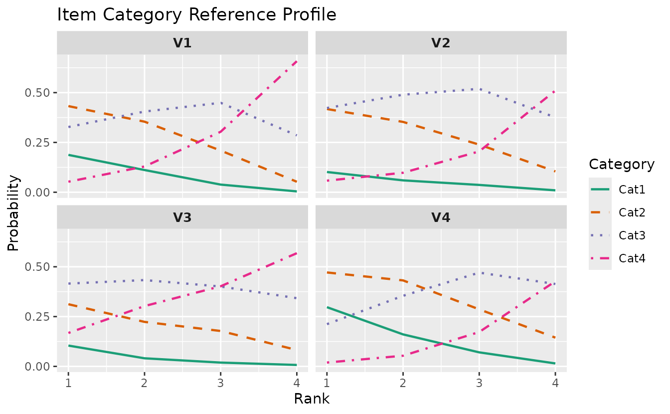
plotICBR_gg: Item Category Boundary Response
Shows cumulative probability curves for each category boundary. For an item with K categories, displays P(response >= k) for k = 1, …, K-1.
icbr_plots <- plotICBR_gg(result_lra_ord, items = 1:4)
icbr_plots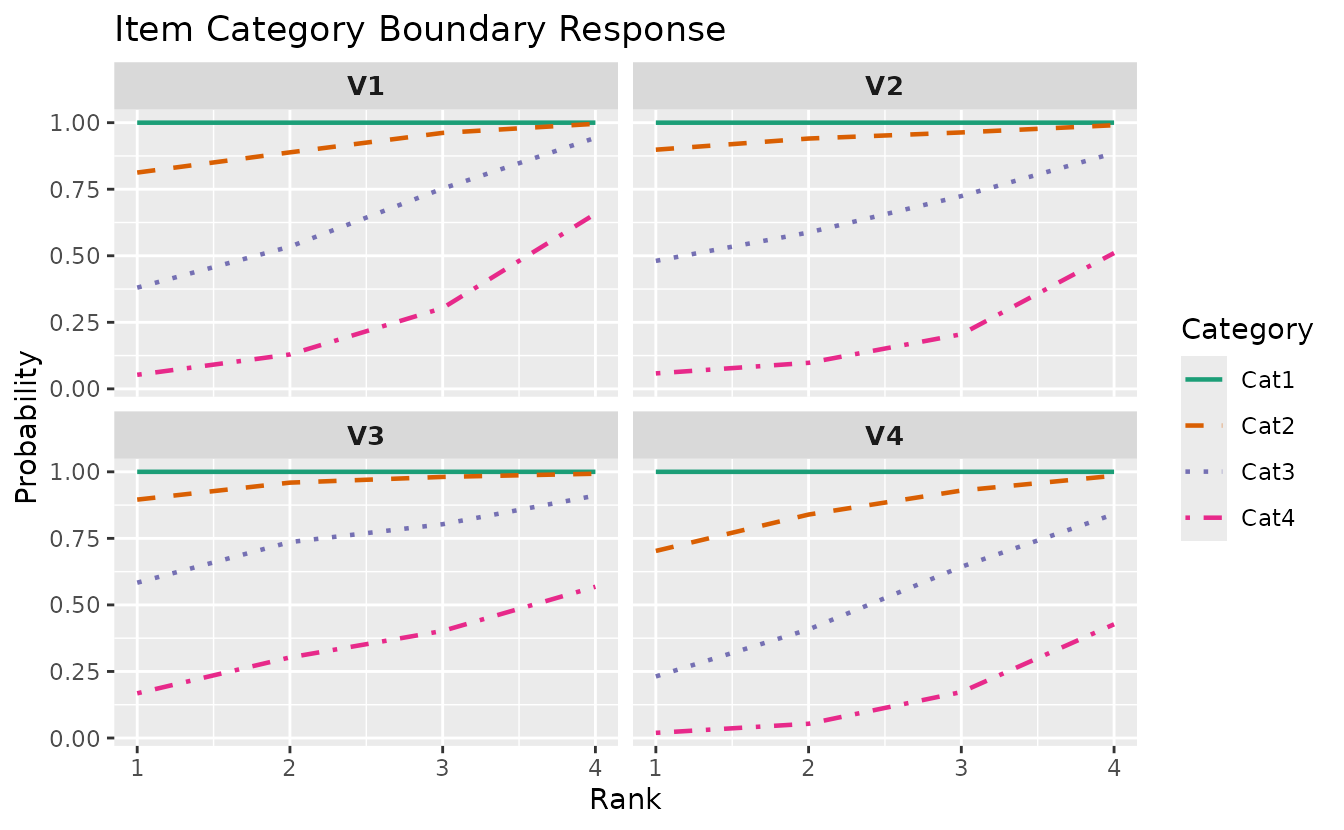
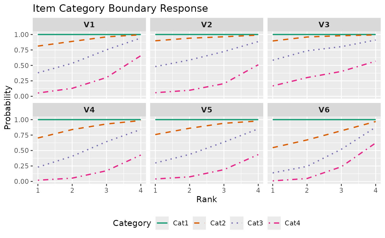
Customize:
plotICBR_gg(result_lra_ord,
  items = 1:6,
  title = "Item Category Boundary Response",
  legend_position = "bottom"
)
plotRMP_gg: Rank Membership Profile
Also works with LRAordinal/LRArated:
rmp_plots <- plotRMP_gg(result_lra_ord)
rmp_plots[[1]]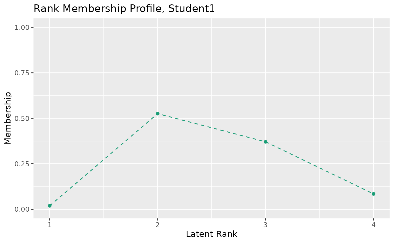
5. Biclustering
Biclustering simultaneously clusters items (into fields) and students (into ranks).
result_bic <- Biclustering(J35S515, nfld = 5, nrank = 6)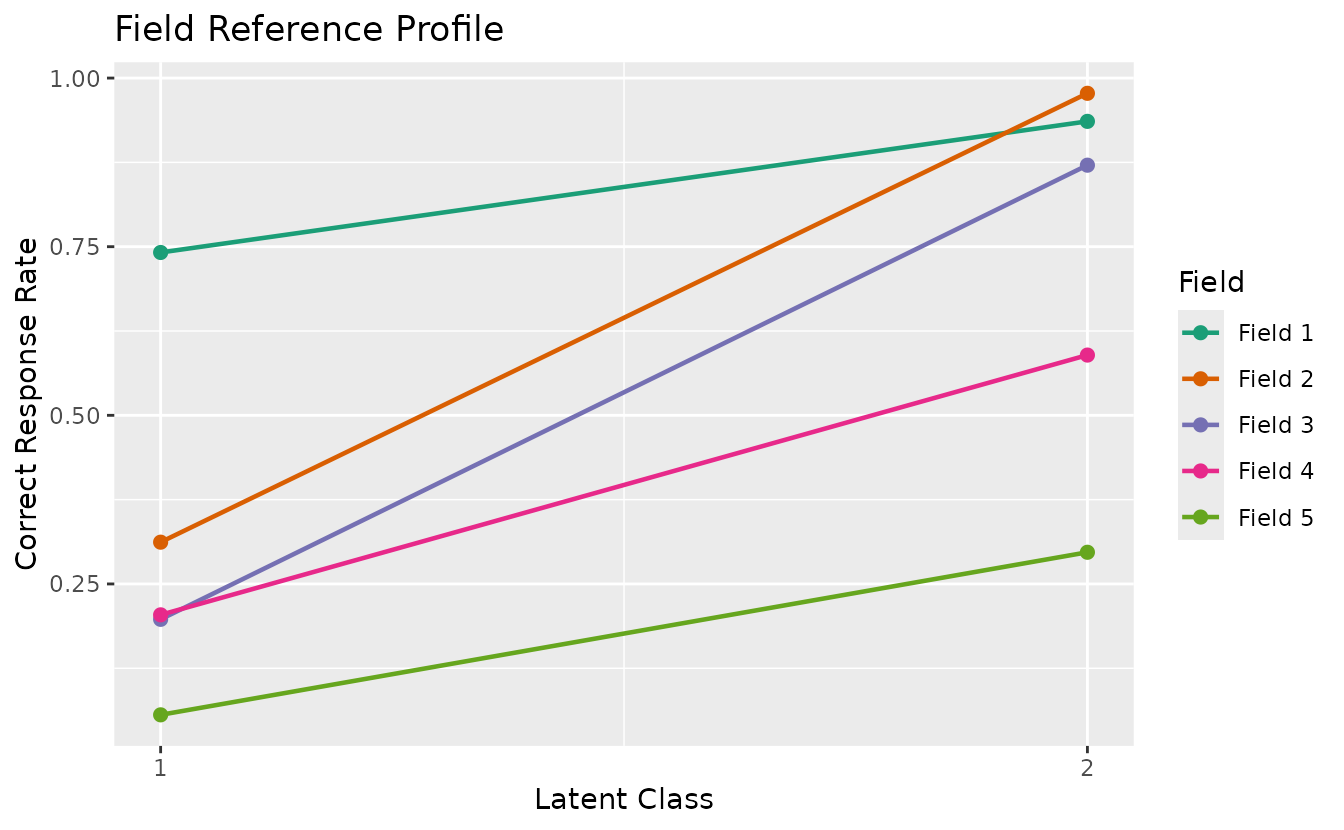
plotRMP_gg: Rank Membership Profile
rmp_plots <- plotRMP_gg(result_bic)
combinePlots_gg(rmp_plots, selectPlots = 1:6)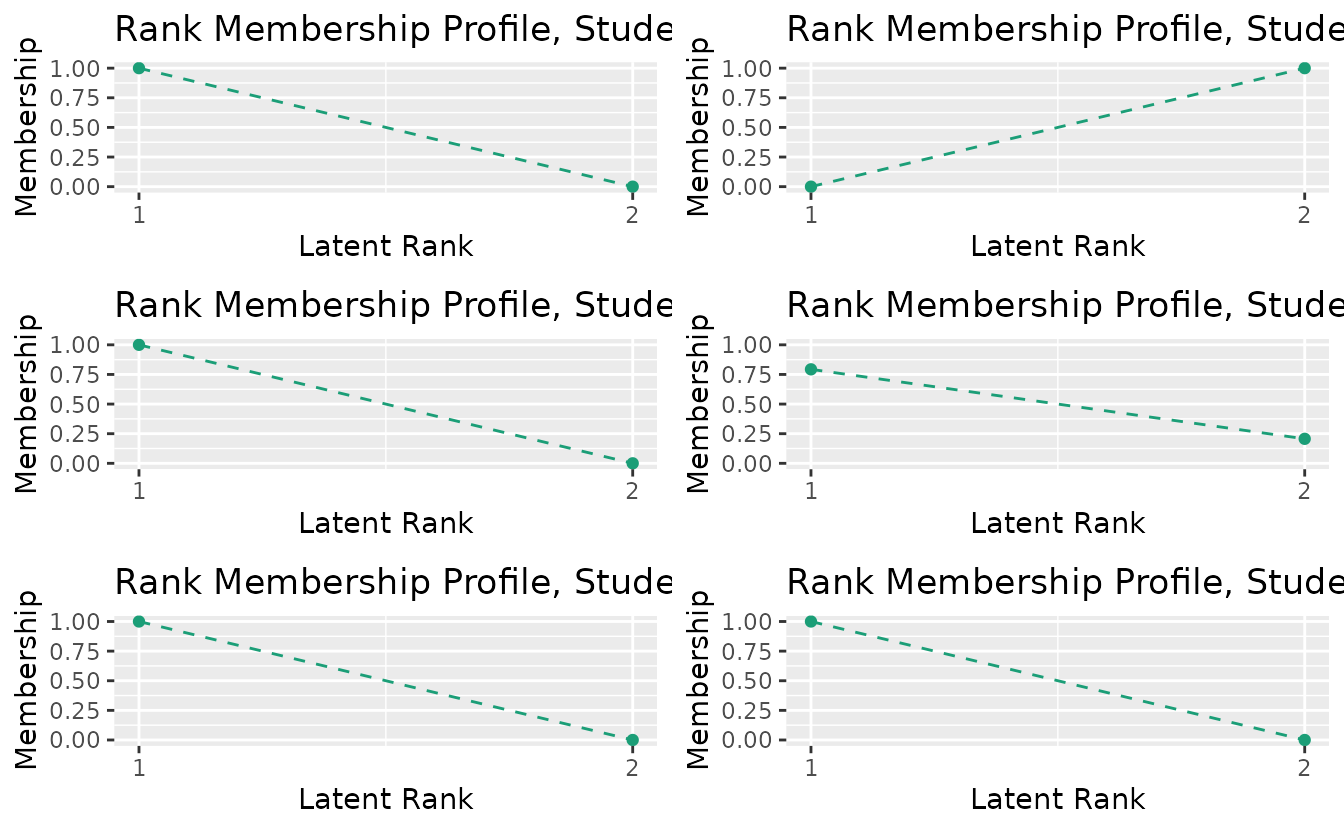
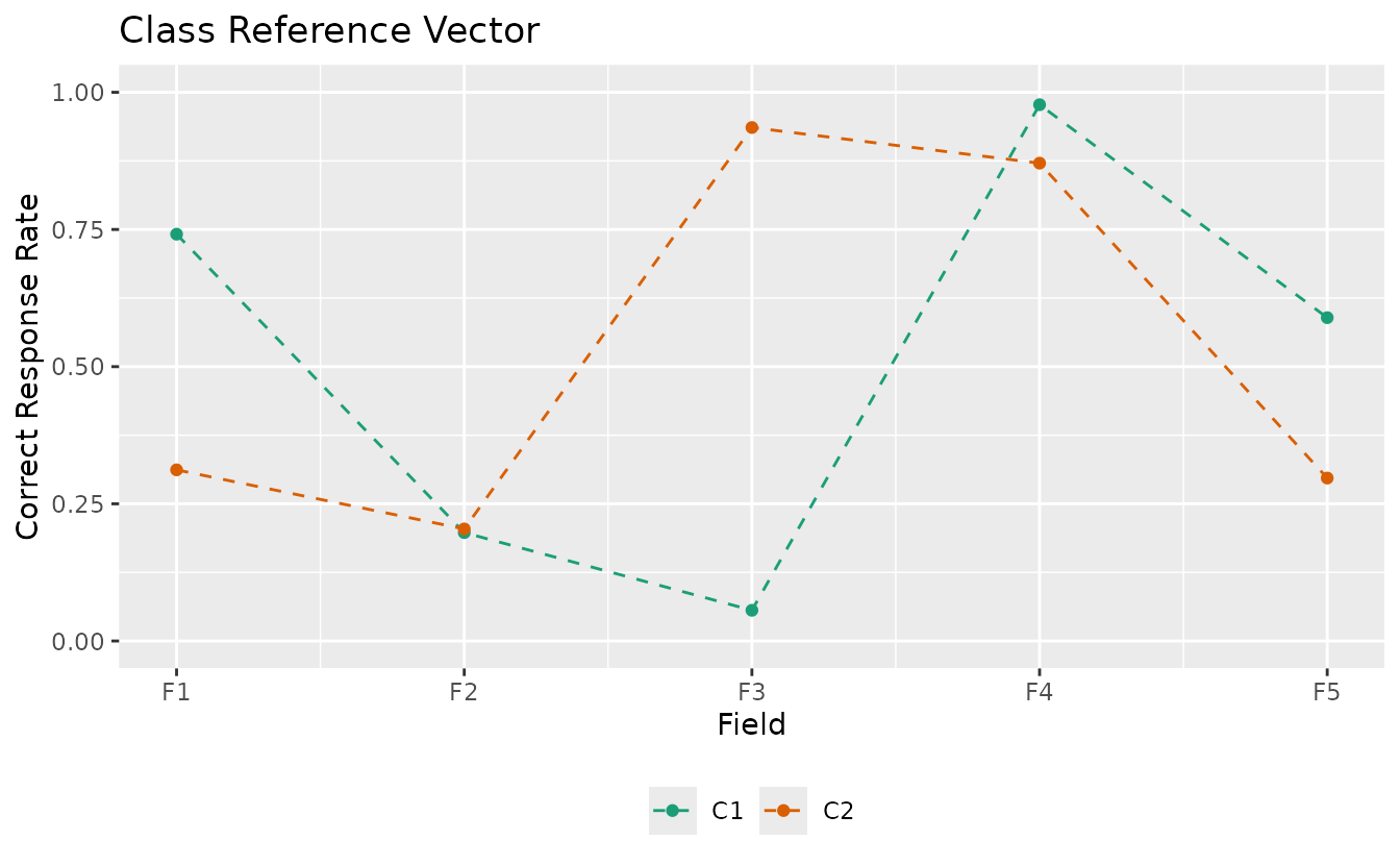
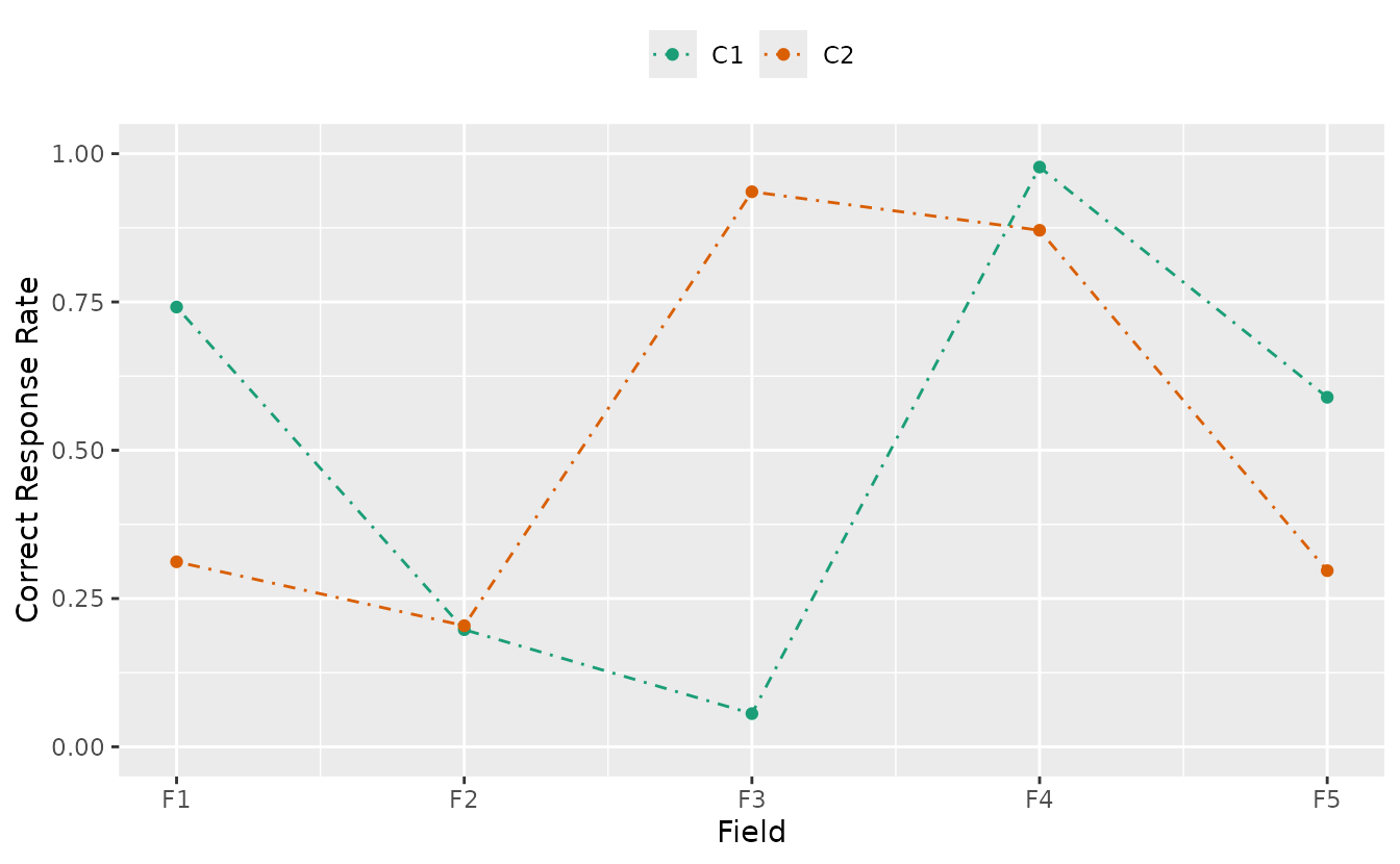
plotCRV_gg: Class Reference Vector
Displays all class profiles in a single plot with one line per class.
crv_plot <- plotCRV_gg(result_bic)
crv_plot
Customize:
plotCRV_gg(result_bic,
  title = "Class Reference Vector",
  linetype = "dashed",
  legend_position = "bottom"
)
plotRRV_gg: Rank Reference Vector
Displays all rank profiles in a single plot with one line per rank.
rrv_plot <- plotRRV_gg(result_bic)
rrv_plot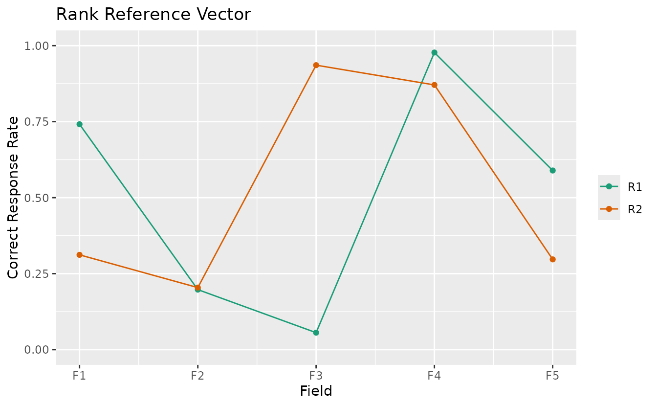
plotArray_gg: Array Plot
Visualizes the binary data matrix as a heatmap, showing the block-diagonal structure after biclustering.
# Show both original and clustered arrays
array_plot <- plotArray_gg(result_bic)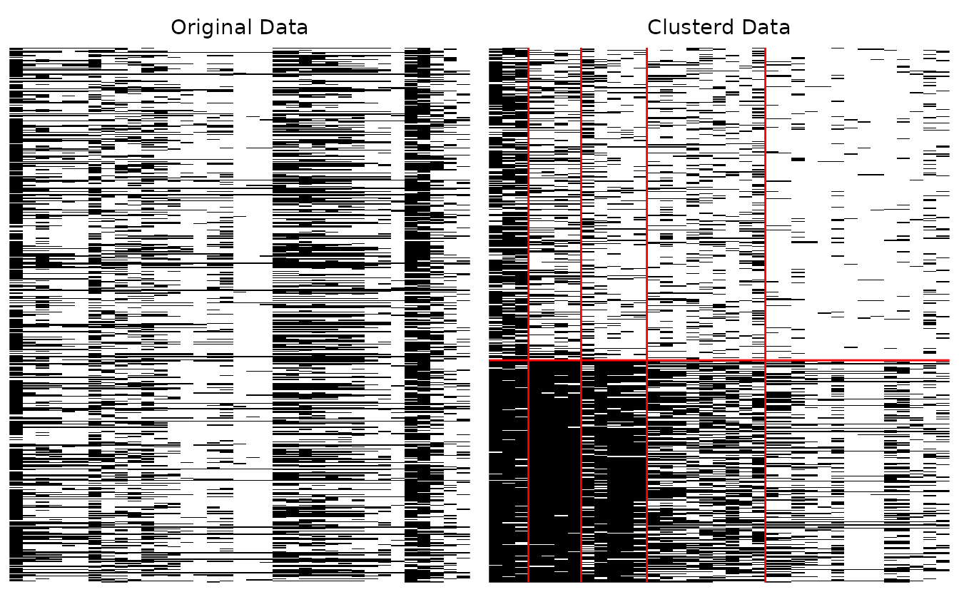
array_plot
#> TableGrob (1 x 2) "arrange": 2 grobs
#>   z     cells    name           grob
#> 1 1 (1-1,1-1) arrange gtable[layout]
#> 2 2 (1-1,2-2) arrange gtable[layout]
Show only the clustered array:
plotArray_gg(result_bic, Original = FALSE, Clustered = TRUE)
#> [[1]]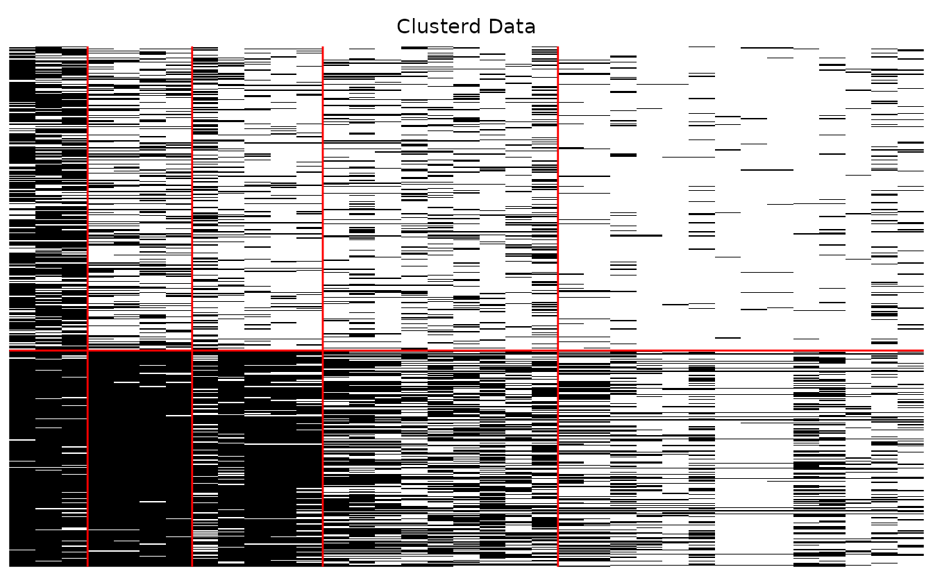
Hide cluster boundary lines:
plotArray_gg(result_bic, Clustered_lines = FALSE)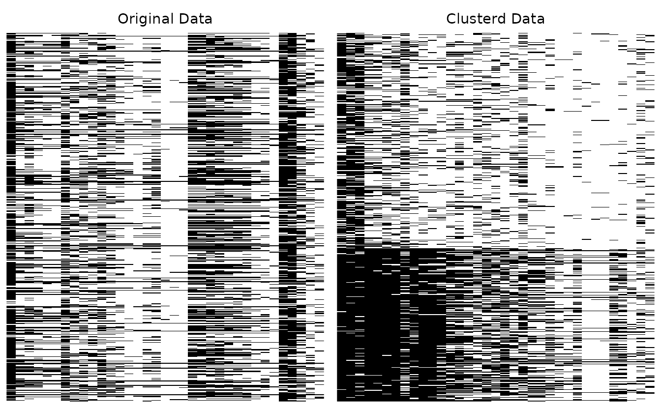
#> TableGrob (1 x 2) "arrange": 2 grobs
#>   z     cells    name           grob
#> 1 1 (1-1,1-1) arrange gtable[layout]
#> 2 2 (1-1,2-2) arrange gtable[layout]
Ordinal Biclustering: plotFCBR_gg
For ordinal (polytomous) biclustering, plotFCBR_gg()
visualizes the Field Cumulative Boundary Reference. It shows boundary
probabilities P(Q >= k) for each field across latent
classes/ranks.
result_ord_bic <- Biclustering(J35S500, ncls = 5, nfld = 5)
fcbr_plot <- plotFCBR_gg(result_ord_bic)
fcbr_plot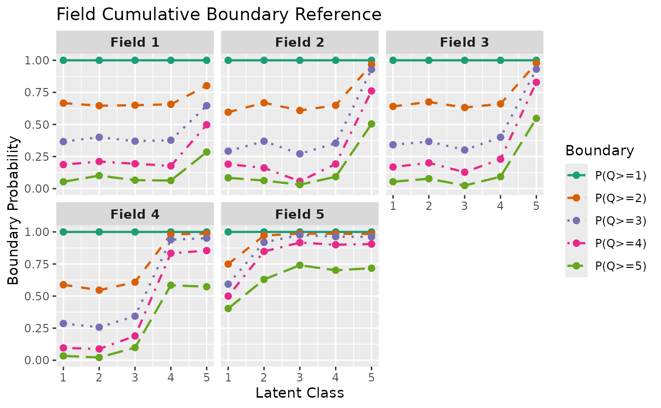
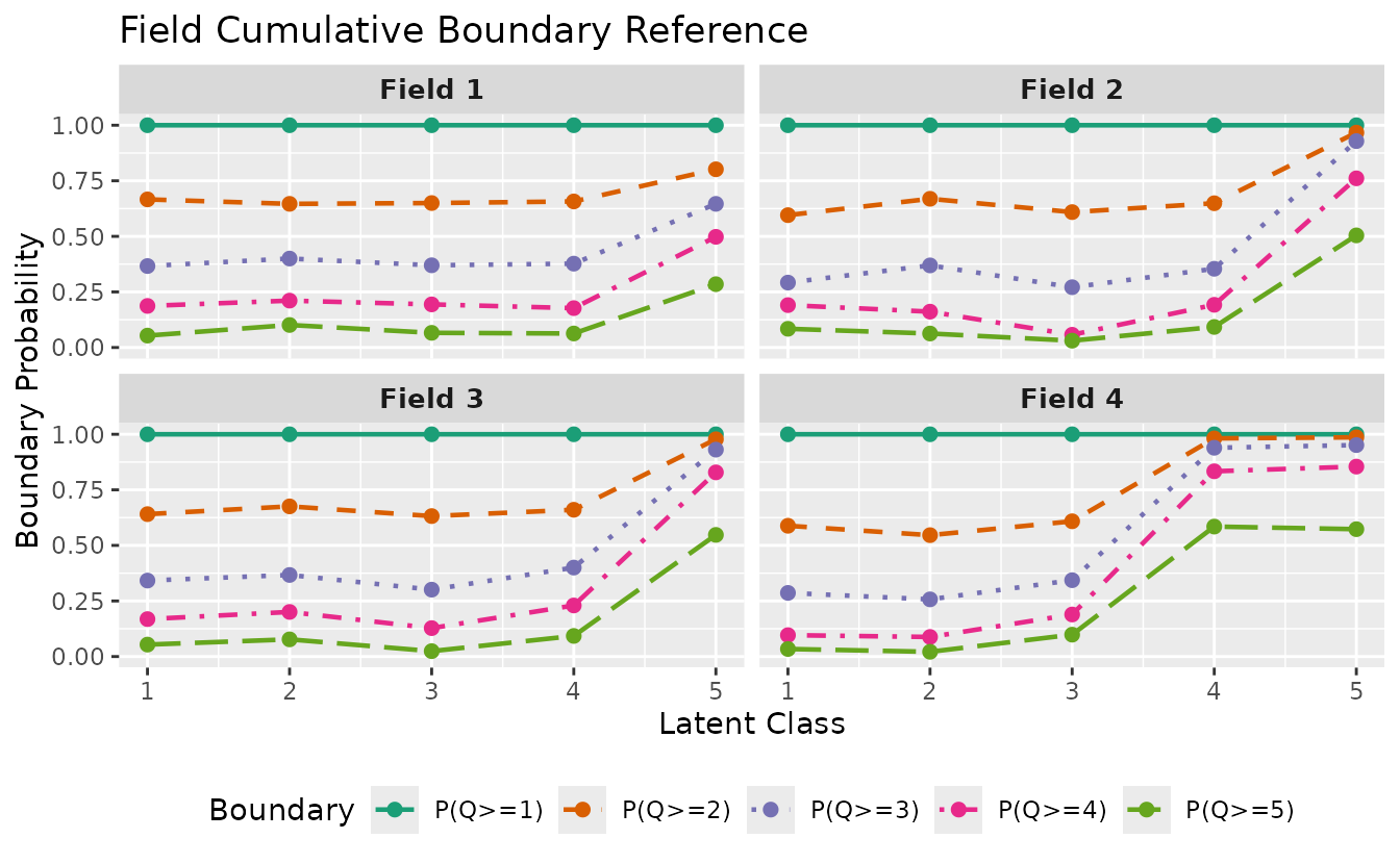
Select specific fields and customize:
plotFCBR_gg(result_ord_bic,
  fields = 1:4,
  title = "Field Cumulative Boundary Reference",
  legend_position = "bottom"
)
6. BNM (Bayesian Network Model)
BNM discovers the dependency structure among items using a Bayesian network.
result_bnm <- BNM(J15S500)plotGraph_gg: DAG Visualization
Visualizes the Directed Acyclic Graph (DAG) discovered by the model.
dag_plots <- plotGraph_gg(result_bnm)
dag_plots[[1]]
Customize layout and appearance:
plotGraph_gg(result_bnm,
  layout = "sugiyama",
  direction = "LR",
  node_size = 10,
  label_size = 4,
  title = "BNM DAG"
)
Available layouts: "sugiyama" (hierarchical),
"fr" (Fruchterman-Reingold), "kk"
(Kamada-Kawai), "tree", "circle",
"grid", "stress".
7. LDLRA (Locally Dependent Latent Rank Analysis)
LDLRA adds local dependency structures within each rank.
result_ldlra <- LDLRA(J15S500, ncls = 5)plotIRP_gg: Item Reference Profile
irp_plots <- plotIRP_gg(result_ldlra)
combinePlots_gg(irp_plots, selectPlots = 1:6)
plotLRD_gg: Latent Rank Distribution
lrd_plot <- plotLRD_gg(result_ldlra)
lrd_plot
plotRMP_gg: Rank Membership Profile
rmp_plots <- plotRMP_gg(result_ldlra)
combinePlots_gg(rmp_plots, selectPlots = 1:6)
plotGraph_gg: DAG per Rank
Returns one DAG per rank, showing how dependencies change across ranks. (DAG visualization for LDLRA is coming soon.)
dag_plots <- plotGraph_gg(result_ldlra)
dag_plots[[1]] # Rank 1 DAG
combinePlots_gg(dag_plots)
8. LDB (Locally Dependent Biclustering)
LDB adds local dependency structures to the biclustering framework.
result_ldb <- LDB(J35S515, ncls = 6, nfld = 5)plotFRP_gg: Field Reference Profile
frp_plot <- plotFRP_gg(result_ldb)
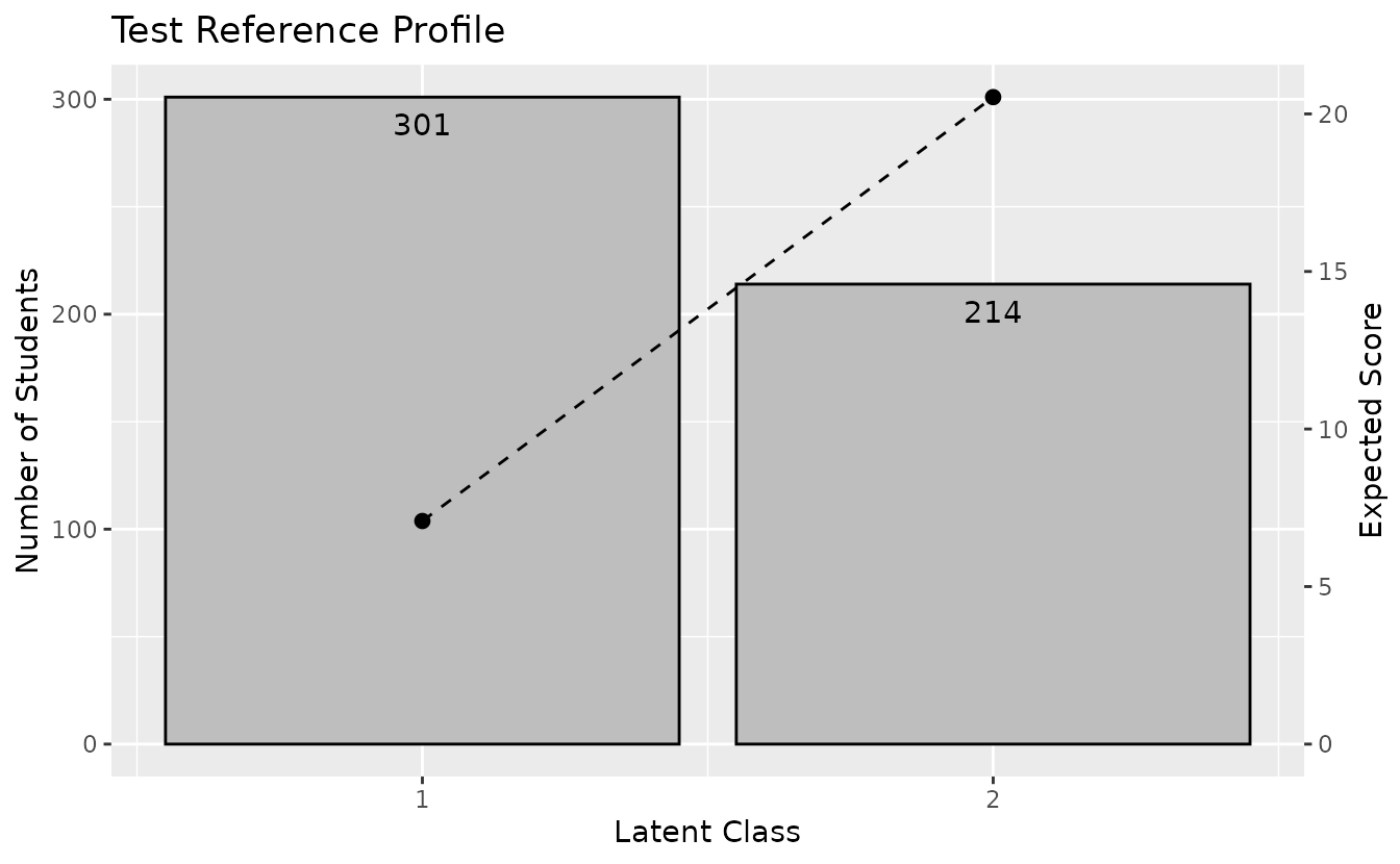
frp_plotplotTRP_gg: Test Reference Profile
trp_plot <- plotTRP_gg(result_ldb)
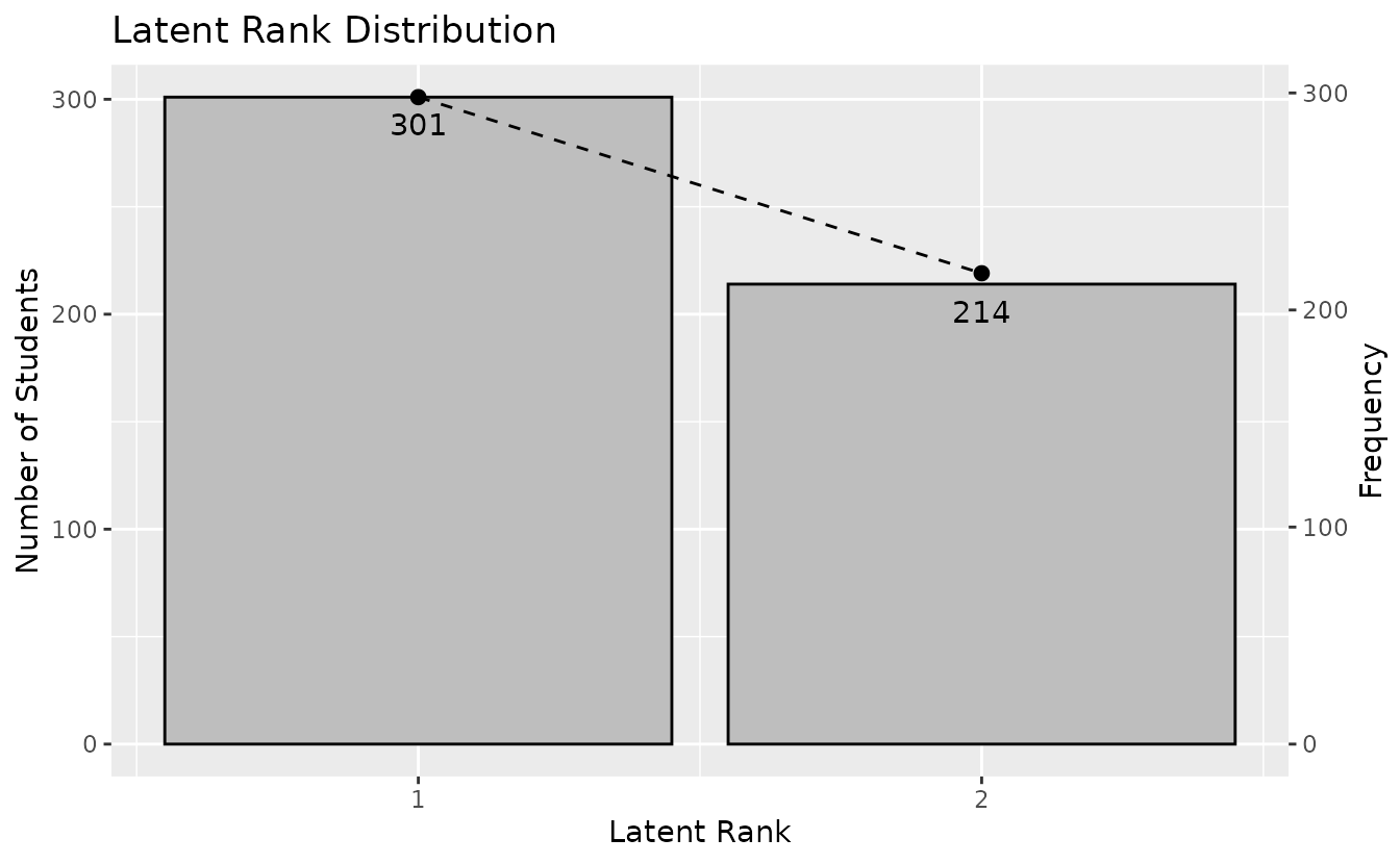
trp_plotplotLRD_gg: Latent Rank Distribution
lrd_plot <- plotLRD_gg(result_ldb)
lrd_plot
plotRMP_gg: Rank Membership Profile
rmp_plots <- plotRMP_gg(result_ldb)
combinePlots_gg(rmp_plots, selectPlots = 1:6)
plotArray_gg: Array Plot
array_plot <- plotArray_gg(result_ldb)
array_plot
plotFieldPIRP_gg: Field Parent Item Reference Profile
Shows how field performance varies based on parent field scores, for each rank.
fpirp_plots <- plotFieldPIRP_gg(result_ldb)
fpirp_plots[[1]] # Rank 1
combinePlots_gg(fpirp_plots)
plotGraph_gg: DAG per Rank
(DAG visualization for LDB is coming soon.)
dag_plots <- plotGraph_gg(result_ldb)
dag_plots[[1]]
combinePlots_gg(dag_plots)
9. BINET (Bayesian Network and Test)
BINET combines Bayesian network structure with the biclustering framework.
result_binet <- BINET(J35S515, ncls = 6, nfld = 5)plotFRP_gg: Field Reference Profile
frp_plot <- plotFRP_gg(result_binet)
frp_plot
plotTRP_gg: Test Reference Profile
trp_plot <- plotTRP_gg(result_binet)
trp_plot
plotLCD_gg: Latent Class Distribution
lcd_plot <- plotLCD_gg(result_binet)
lcd_plot
plotCMP_gg: Class Membership Profile
cmp_plots <- plotCMP_gg(result_binet)
combinePlots_gg(cmp_plots, selectPlots = 1:6)
plotArray_gg: Array Plot
array_plot <- plotArray_gg(result_binet)
array_plot
plotGraph_gg: DAG Visualization
BINET supports edge labels showing dependency weights. (DAG visualization for BINET is coming soon.)
dag_plots <- plotGraph_gg(result_binet)
dag_plots[[1]]
10. Common Plot Options
Many functions support the following options for customization:
| Parameter | Description | Default |
|---|---|---|
title |
TRUE (auto), FALSE (none), or character
string |
TRUE |
colors |
Color vector for lines/bars | Colorblind-friendly palette |
linetype |
Line type ("solid", "dashed",
"dotted", etc.) |
"solid" |
show_legend |
Show/hide legend | TRUE |
legend_position |
"right", "top", "bottom",
"left", "none"
|
"right" |
Example: Customizing plotICRF_gg
plotICRF_gg(result_grm,
  items = 1,
  title = "Custom ICRF Title",
  colors = c("#E41A1C", "#377EB8", "#4DAF4A", "#984EA3", "#FF7F00"),
  linetype = "dashed",
  show_legend = TRUE,
  legend_position = "bottom"
)
#> [[1]]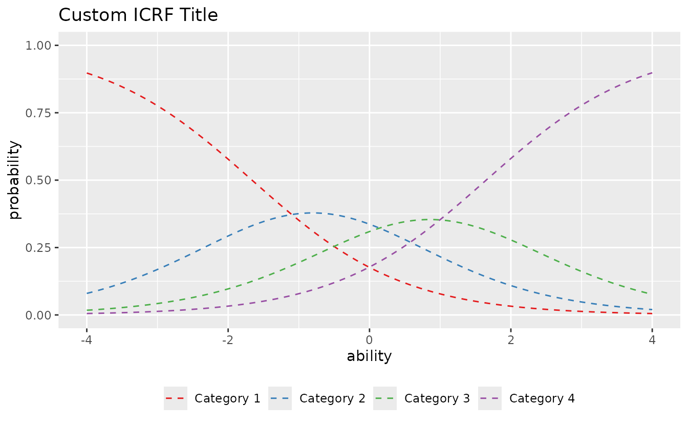
Example: Customizing plotCRV_gg
plotCRV_gg(result_bic,
  title = FALSE,
  linetype = "dotdash",
  show_legend = TRUE,
  legend_position = "top"
)
11. combinePlots_gg: Arranging Multiple Plots
combinePlots_gg() arranges multiple ggplot objects in a
grid layout.
# Default: first 6 plots
plots <- plotICC_gg(result_irt)
combinePlots_gg(plots)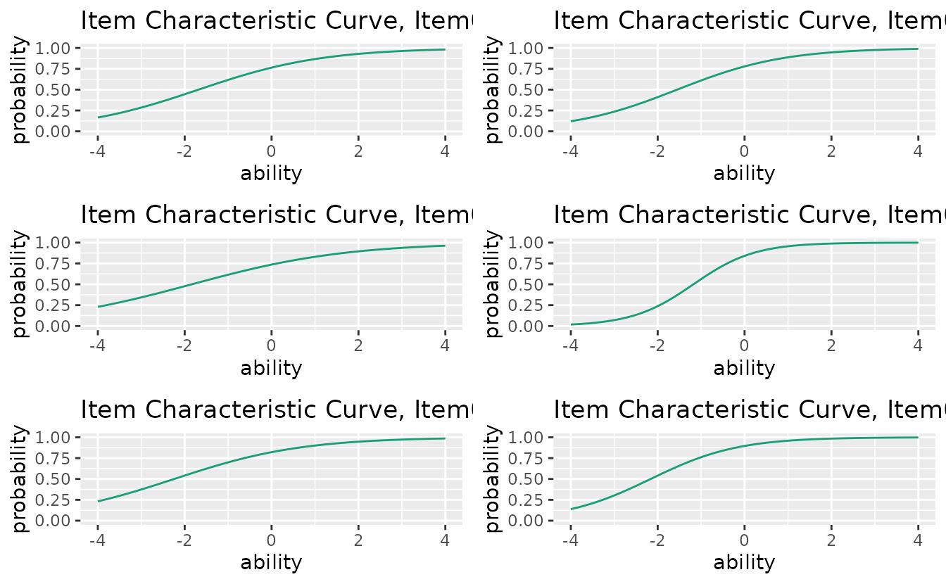
# Select specific plots
combinePlots_gg(plots, selectPlots = c(1, 3, 5, 7))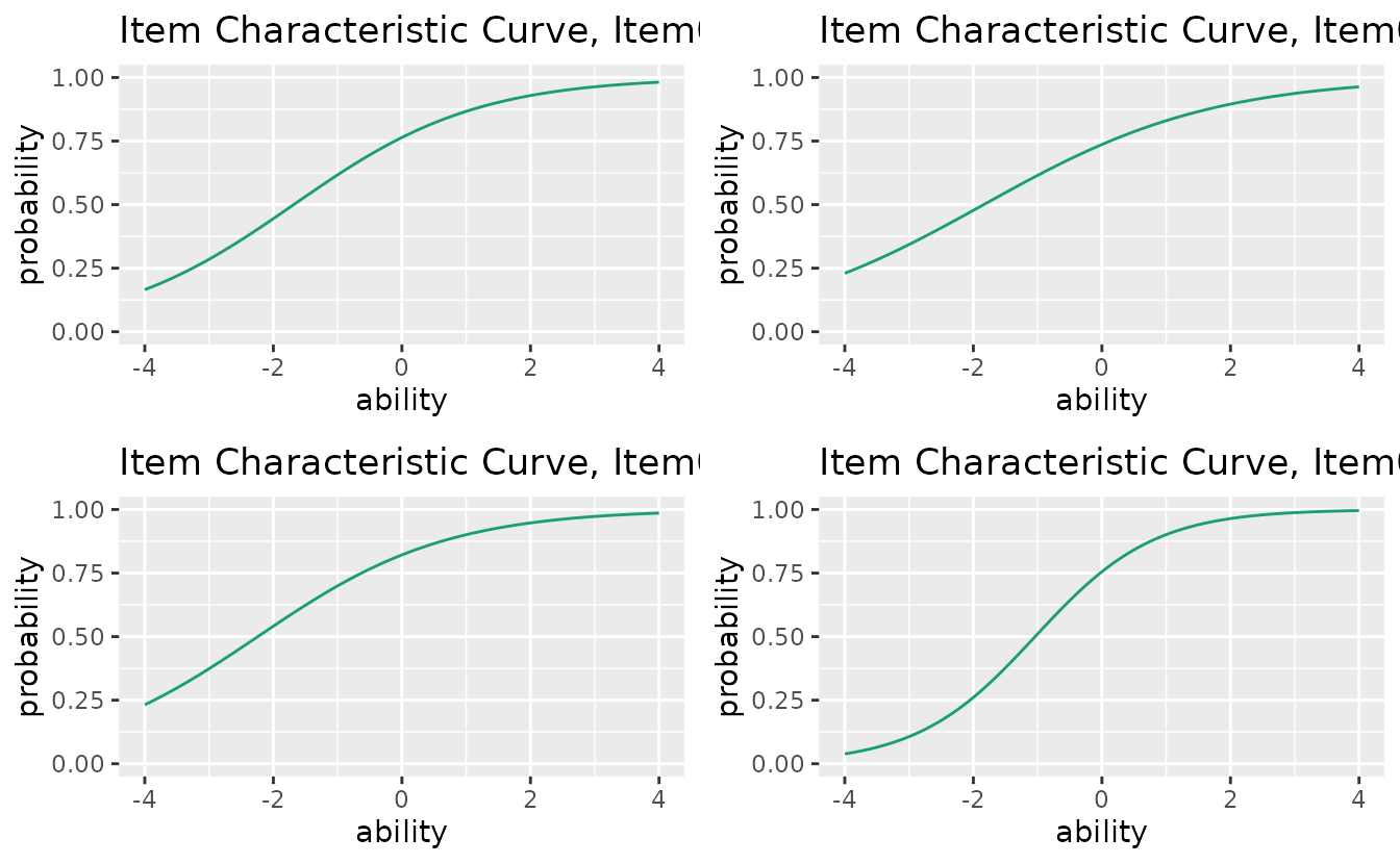
# All 15 items
combinePlots_gg(plots, selectPlots = 1:15)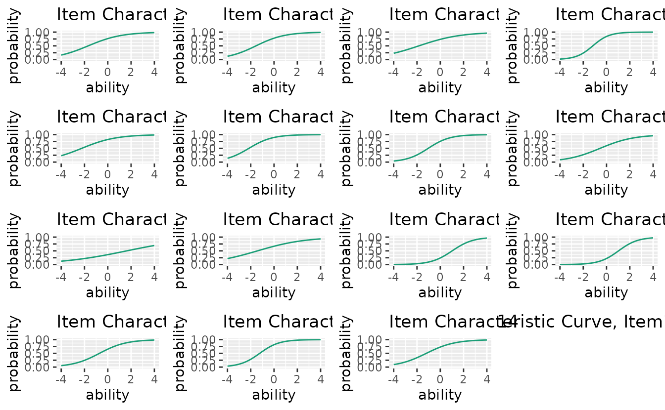
Function-Model Compatibility Matrix
| Function | IRT | GRM | LCA | LRA | LRAord | LRArat | Biclust | nomBiclust | ordBiclust | IRM | LDLRA | LDB | BINET | BNM |
|---|---|---|---|---|---|---|---|---|---|---|---|---|---|---|
| plotICC_gg | x | |||||||||||||
| plotICC_overlay_gg | x | |||||||||||||
| plotIIC_gg | x | x | ||||||||||||
| plotIIC_overlay_gg | x | x | ||||||||||||
| plotTIC_gg | x | x | ||||||||||||
| plotTRF_gg | x | |||||||||||||
| plotICRF_gg | x | |||||||||||||
| plotIRP_gg | x | x | x | |||||||||||
| plotFRP_gg | x | x | x | x | x | x | ||||||||
| plotTRP_gg | x | x | x | x | x | x | x | |||||||
| plotLCD_gg | x | x | ||||||||||||
| plotLRD_gg | x | x | x | x | x | x | ||||||||
| plotCMP_gg | x | x | ||||||||||||
| plotRMP_gg | x | x | x | x | x | x | x | x | ||||||
| plotCRV_gg | x | x | x | |||||||||||
| plotRRV_gg | x | x | x | |||||||||||
| plotArray_gg | x | x | x | x | x | x | ||||||||
| plotFieldPIRP_gg | x | |||||||||||||
| plotGraph_gg | x | x | x | x | ||||||||||
| plotScoreFreq_gg | x | x | ||||||||||||
| plotScoreRank_gg | x | x | ||||||||||||
| plotICRP_gg | x | x | ||||||||||||
| plotICBR_gg | x | |||||||||||||
| plotFCBR_gg | x | |||||||||||||
| plotFCRP_gg | x | x | ||||||||||||
| plotScoreField_gg | x | x | ||||||||||||
| plotLDPSR_gg | x |