This gallery showcases every visualization function in
ggExametrika. Each plot is generated from real model
output using the exametrika package.
All functions return standard ggplot objects, so you can further
customize them with + theme(), + labs(),
etc.
Model Fitting
We fit all models up front.
# --- IRT (binary, 15 items, 500 students) ---
result_irt <- IRT(J15S500, model = 2)

# --- GRM (ordinal, 5 items, 1000 students) ---
result_grm <- GRM(J5S1000)

# --- LCA (binary, 15 items, 500 students, 3 classes) ---
result_lca <- LCA(J15S500, ncls = 3)

# --- LRA (binary, 15 items, 500 students, 4 ranks) ---
result_lra <- LRA(J15S500, nrank = 4)

# --- LRAordinal (ordinal, 15 items, 3810 students, 4 ranks) ---
result_lra_ord <- LRA(J15S3810, nrank = 4, dataType = "ordinal")

# --- Biclustering: binary (35 items, 515 students) ---
result_bic <- Biclustering(J35S515, nfld = 5, nrank = 6)

# --- Biclustering: ordinal (35 items, 500 students, 5 categories) ---
result_ord_bic <- Biclustering(J35S500, ncls = 5, nfld = 5)

# --- Biclustering: nominal (20 items, 600 students, 4 categories) ---
result_nom_bic <- Biclustering(J20S600, ncls = 5, nfld = 4)
Network models (BNM, LDLRA, LDB, BINET) require explicit graph structure input (an igraph DAG or edge CSV file).
# --- BNM (5 items, 10 students, simple DAG) ---
bnm_dag <- igraph::make_empty_graph(n = 5, directed = TRUE)
igraph::V(bnm_dag)$name <- J5S10$ItemLabel
bnm_dag <- igraph::add_edges(bnm_dag, c(1, 3, 2, 4, 3, 5))
result_bnm <- BNM(J5S10, g = bnm_dag)

# --- LDLRA (12 items, 5000 students, 3 ranks, same DAG per rank) ---
ldlra_g <- igraph::graph_from_data_frame(
  data.frame(
    from = c("Item01", "Item02", "Item03"),
    to = c("Item02", "Item03", "Item04")
  ),
  directed = TRUE
)
result_ldlra <- LDLRA(J12S5000,
  ncls = 3,
  g = list(ldlra_g, ldlra_g, ldlra_g)
)

# --- LDB (35 items, 515 students, 3 fields, 3 ranks) ---
ldb_conf <- rep(1:3, length.out = 35)
ldb_g <- igraph::graph_from_data_frame(
  data.frame(
    from = c("Field01", "Field02"),
    to = c("Field02", "Field03")
  ),
  directed = TRUE
)
result_ldb <- LDB(J35S515,
  ncls = 3, conf = ldb_conf,
  g_list = list(ldb_g, ldb_g, ldb_g)
)

# --- BINET (35 items, 515 students, 3 classes, 3 fields) ---
binet_edges <- data.frame(
  From  = c(1, 2, 1, 2, 1, 2),
  To    = c(2, 3, 2, 3, 2, 3),
  Field = c(1, 1, 2, 2, 3, 3)
)
binet_edge_file <- tempfile(fileext = ".csv")
write.csv(binet_edges, binet_edge_file, row.names = FALSE)
result_binet <- BINET(J35S515,
  ncls = 3, nfld = 3,
  conf = ldb_conf, adj_file = binet_edge_file,
  verbose = FALSE
)
unlink(binet_edge_file)
1. IRT Models
Item Response Theory (2PL, 3PL, 4PL) visualization for binary response data. Data: J15S500 (15 items, 500 students).
plotICC_gg — Item Characteristic Curve
Probability of a correct response as a function of ability (). Returns a list of plots (one per item).
icc_plots <- plotICC_gg(result_irt)
icc_plots[[1]]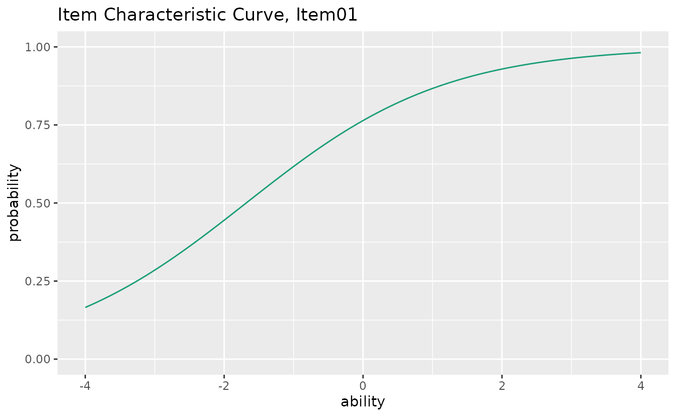
combinePlots_gg(icc_plots, selectPlots = 1:6)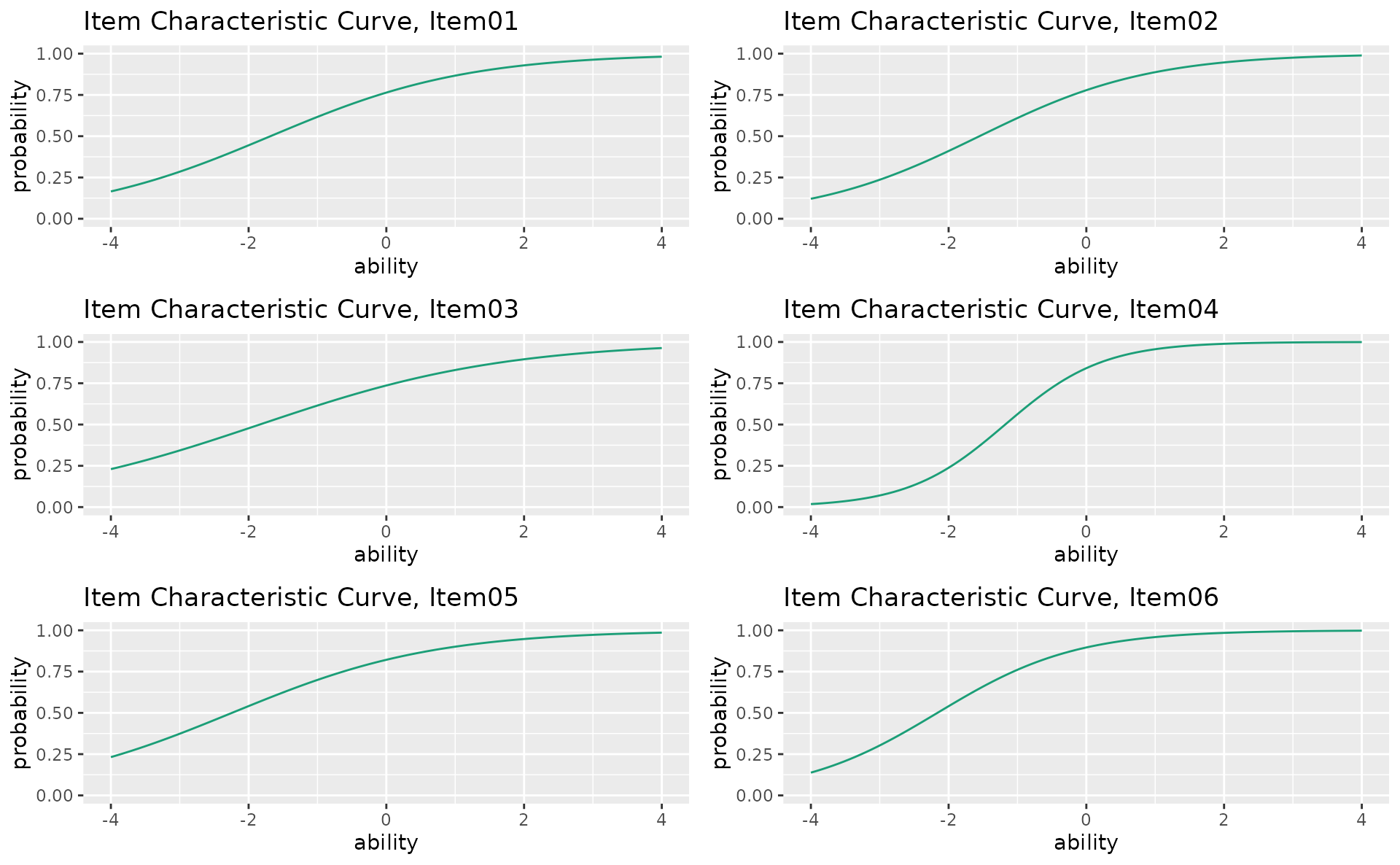
plotICC_overlay_gg — ICC Overlay
All item curves overlaid on a single plot for easy comparison.
plotICC_overlay_gg(result_irt)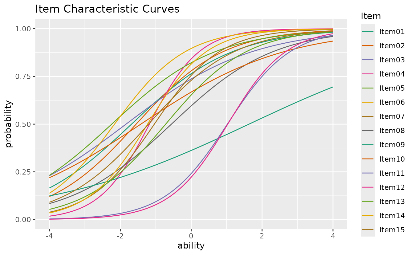
plotIIC_gg — Item Information Curve
How precisely each item measures ability at different levels.
iic_plots <- plotIIC_gg(result_irt)
iic_plots[[1]]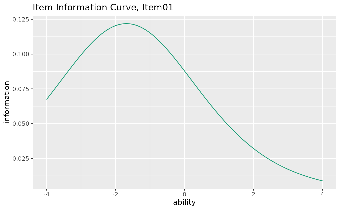
combinePlots_gg(iic_plots, selectPlots = 1:6)
plotIIC_overlay_gg — IIC Overlay
All item information curves on a single plot.
plotIIC_overlay_gg(result_irt)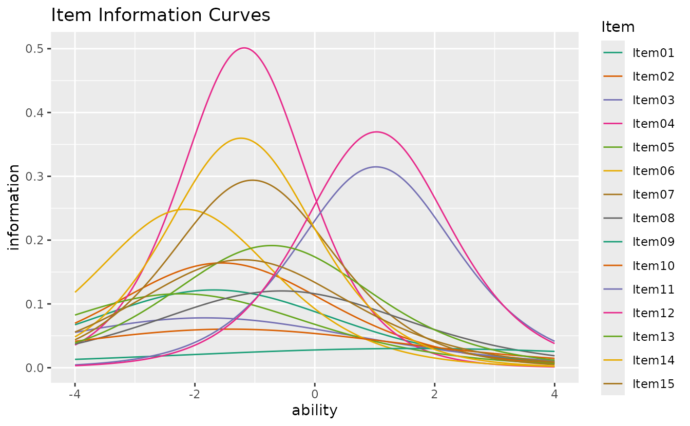
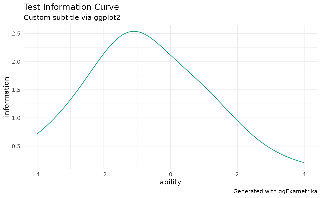
plotTIC_gg — Test Information Curve
Total test information (sum of all item information functions).
plotTIC_gg(result_irt)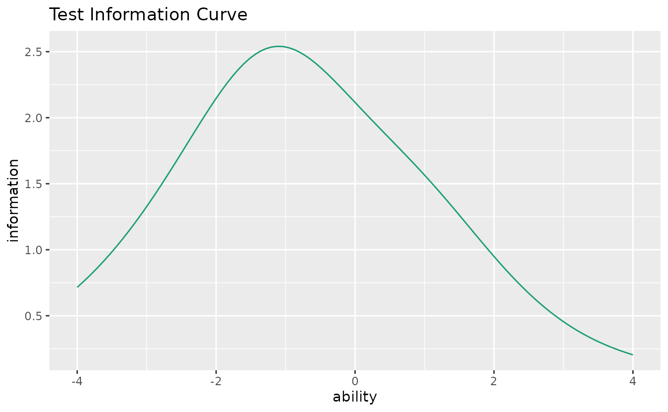
plotTRF_gg — Test Response Function
Expected total score as a function of ability.
plotTRF_gg(result_irt)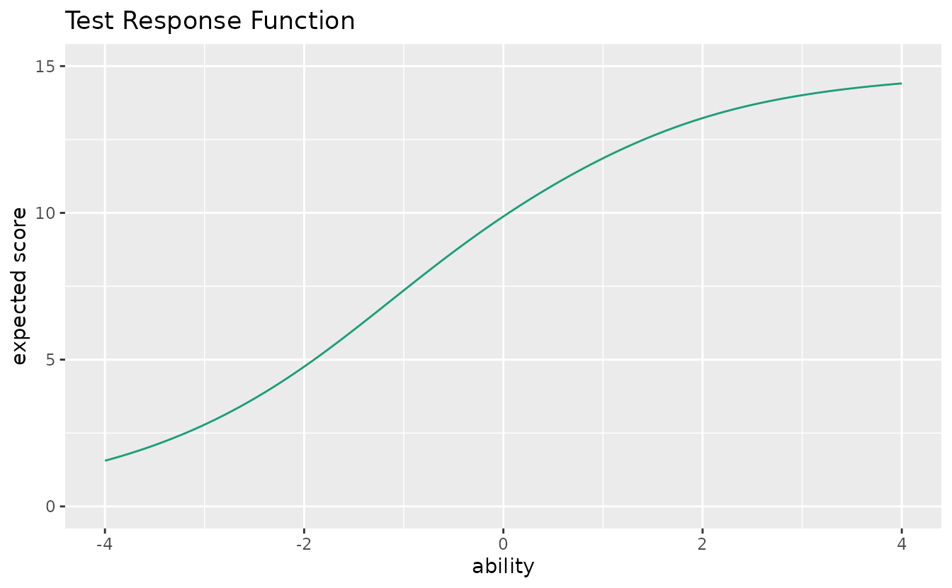
2. GRM (Graded Response Model)
Visualization for ordered polytomous response data. Data: J5S1000 (5 items, 1000 students).
plotICRF_gg — Item Category Response Function
Probability of each response category as a function of ability. Returns a list of plots (one per item).
icrf_plots <- plotICRF_gg(result_grm)
icrf_plots[[1]]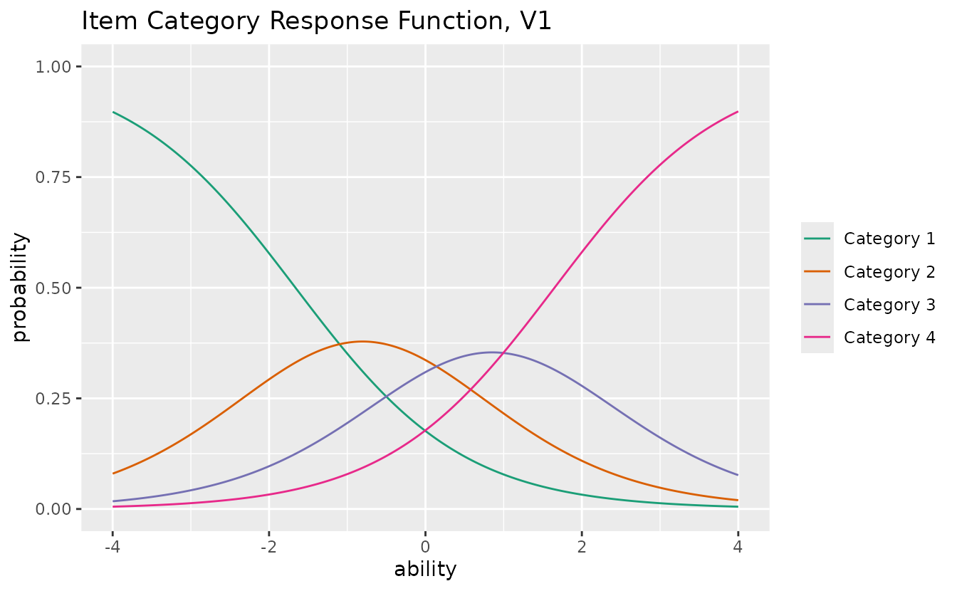
combinePlots_gg(icrf_plots, selectPlots = 1:5)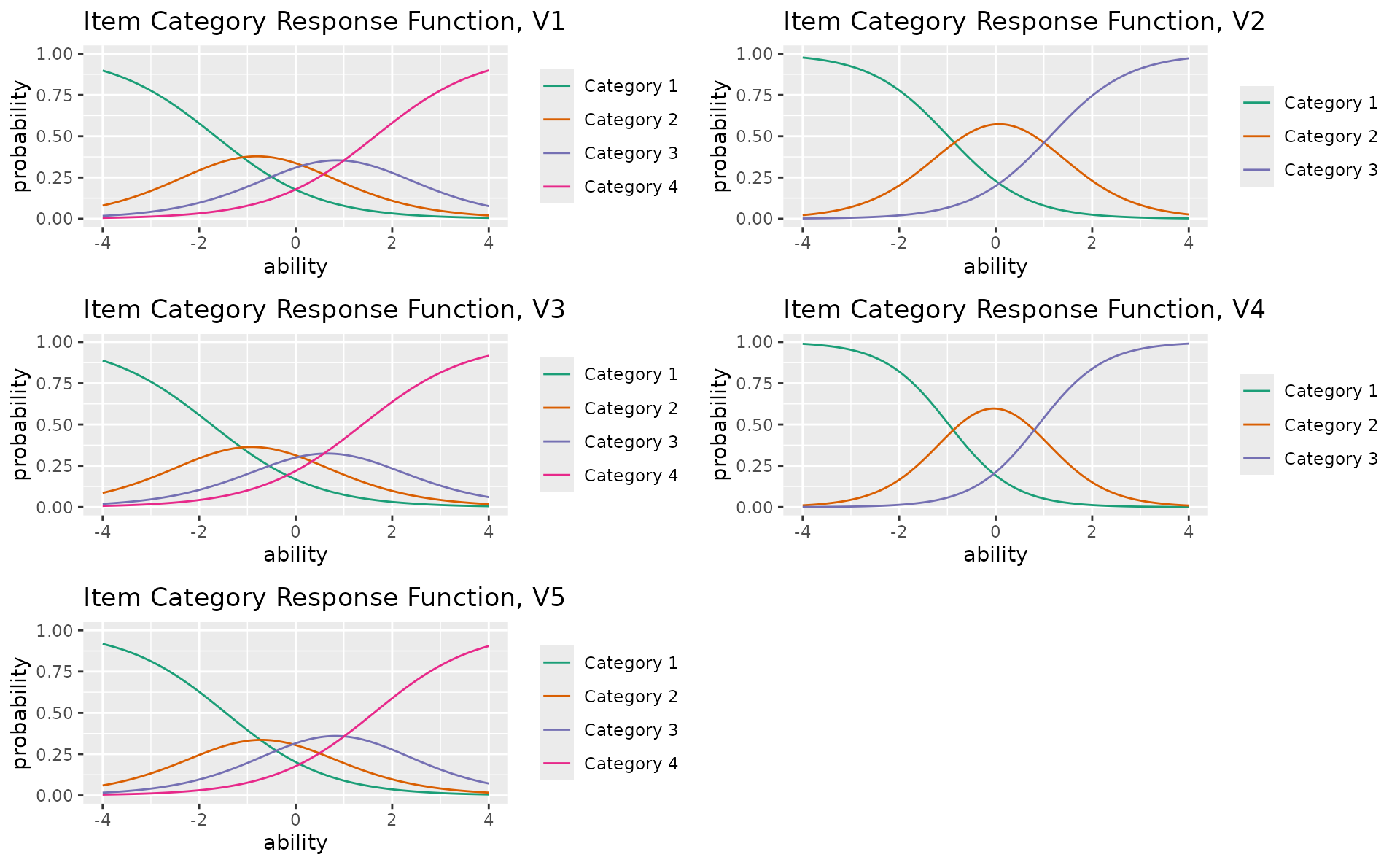
Note:
plotIIC_gg()andplotTIC_gg()also accept GRM output. See the Getting Started vignette for examples.
3. Latent Class / Rank Analysis
Visualization for discrete latent variable models. Data: J15S500 with LCA (3 classes) and LRA (4 ranks).
plotIRP_gg — Item Reference Profile
Probability of a correct response for each item within each latent class or rank. Returns a list of plots (one per item).
irp_plots <- plotIRP_gg(result_lca)
irp_plots[[1]]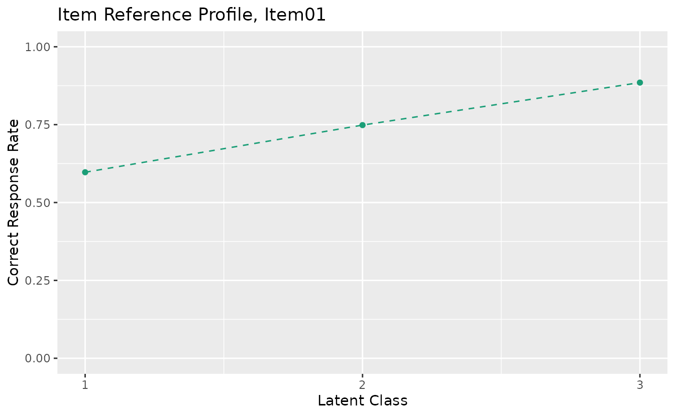
combinePlots_gg(irp_plots, selectPlots = 1:6)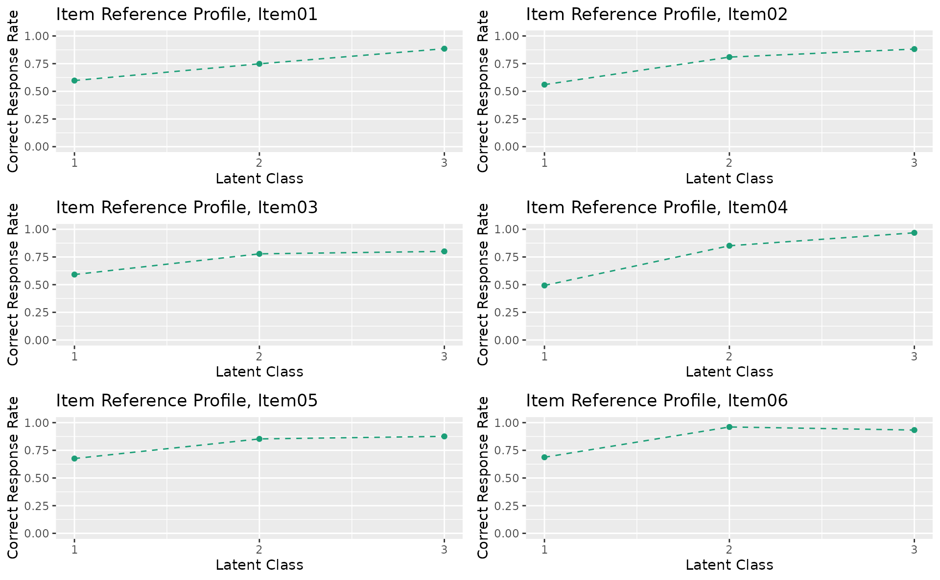
plotFRP_gg — Field Reference Profile
Correct response rate by field for each class/rank. Returns a list of plots (one per field).
Note:
plotFRP_gg()requires a model with field structure (Biclustering, IRM, LDB, or BINET). Shown here with binary Biclustering on J35S515 (5 fields, 6 ranks).
plotFRP_gg(result_bic)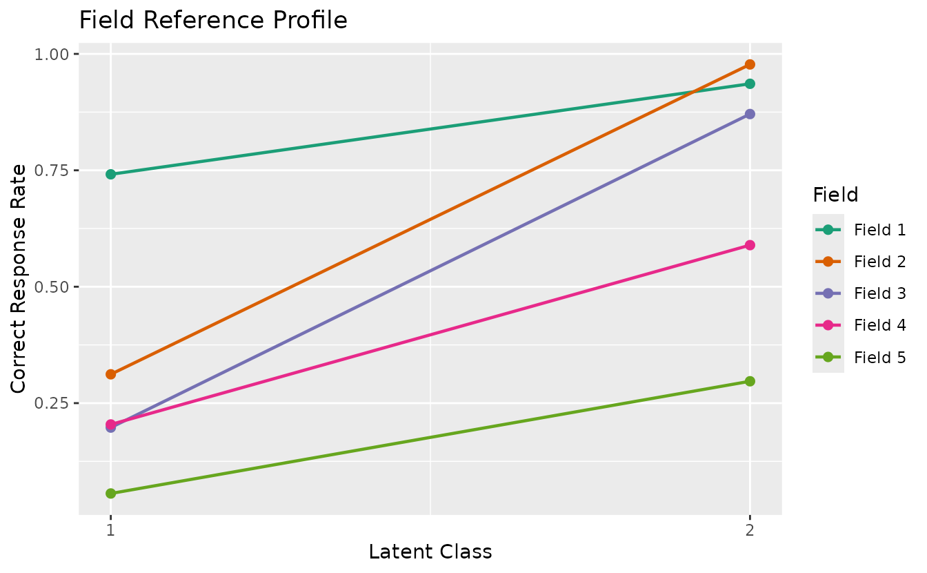
plotTRP_gg — Test Reference Profile
Number of students and expected test score per class/rank.
plotTRP_gg(result_lca)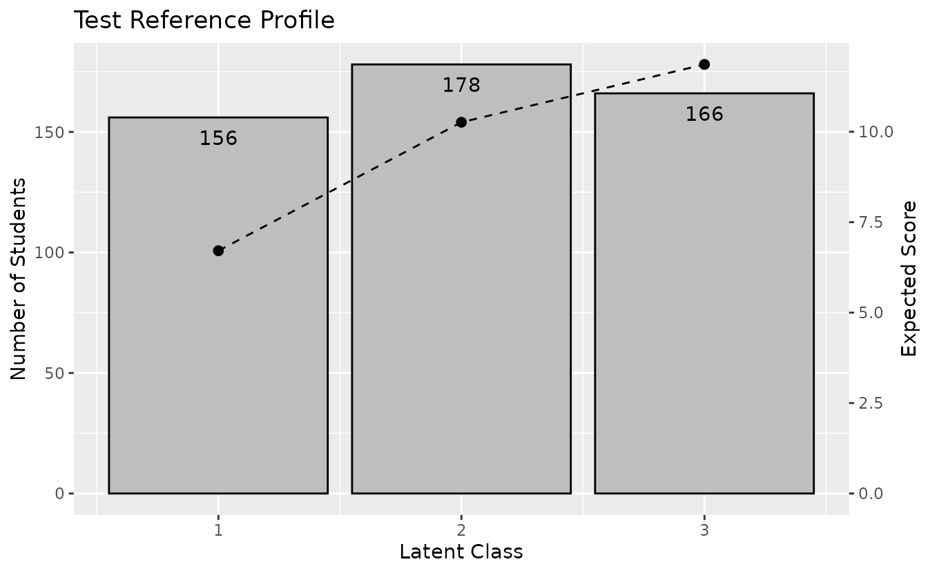
plotCMP_gg — Class Membership Profile
Membership probability profile for each student across all classes. Returns a list of plots (one per student).
cmp_plots <- plotCMP_gg(result_lca)
combinePlots_gg(cmp_plots, selectPlots = 1:6)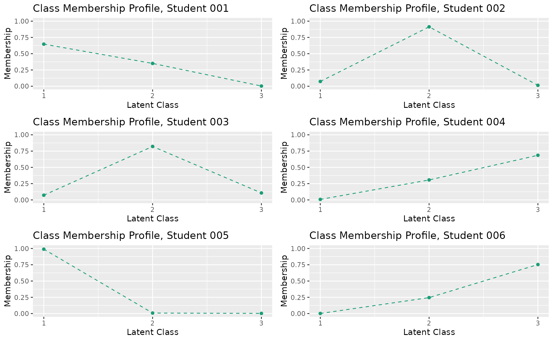
plotRMP_gg — Rank Membership Profile
Membership probability profile for each student across all ranks. Returns a list of plots (one per student).
rmp_plots <- plotRMP_gg(result_lra)
combinePlots_gg(rmp_plots, selectPlots = 1:6)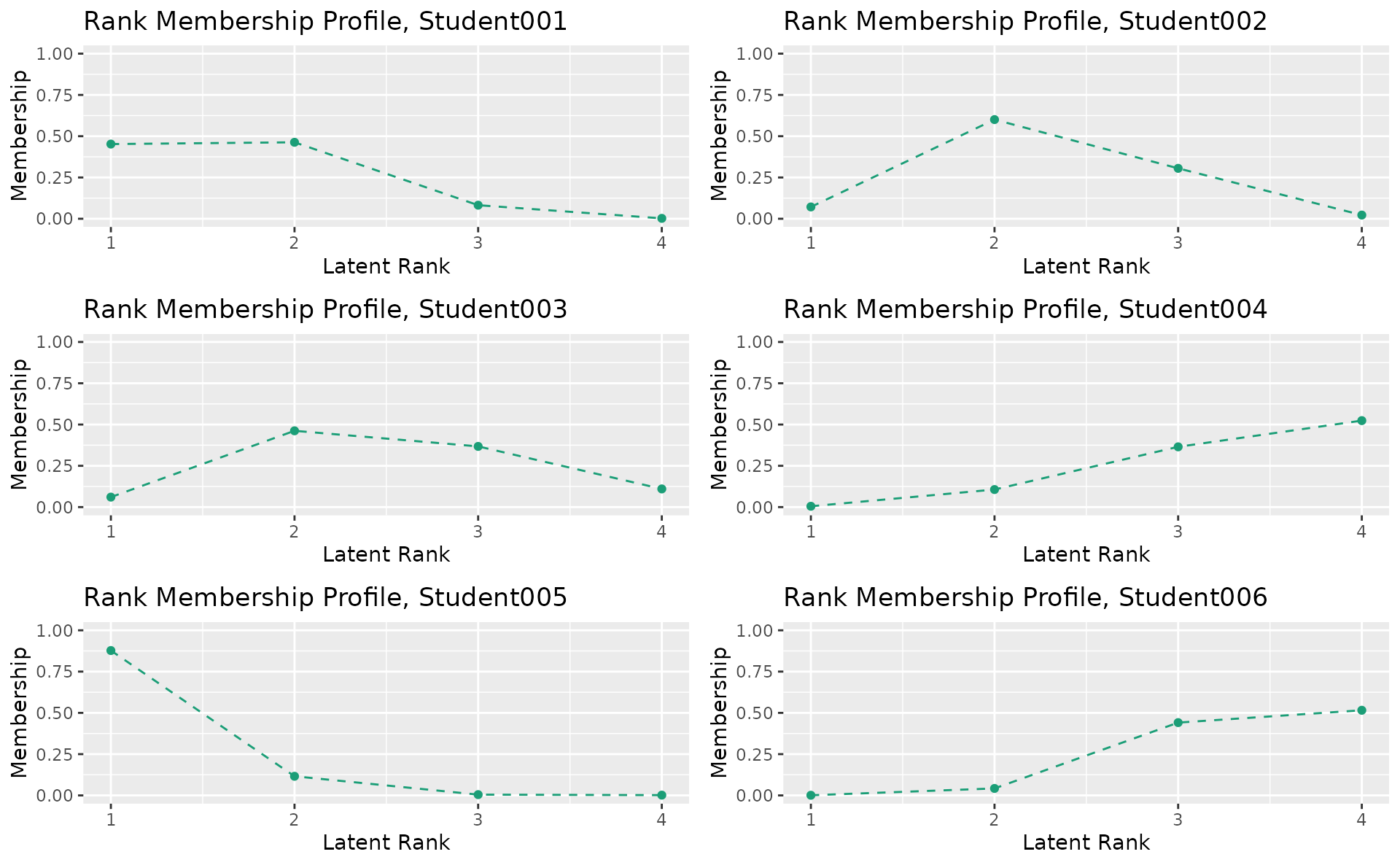
4. Biclustering
Biclustering simultaneously clusters items (into fields) and students (into ranks/classes). This section covers binary, ordinal, and nominal Biclustering visualizations.
Binary Biclustering
Data: J35S515 (35 items, 515 students, 5 fields, 6 ranks).
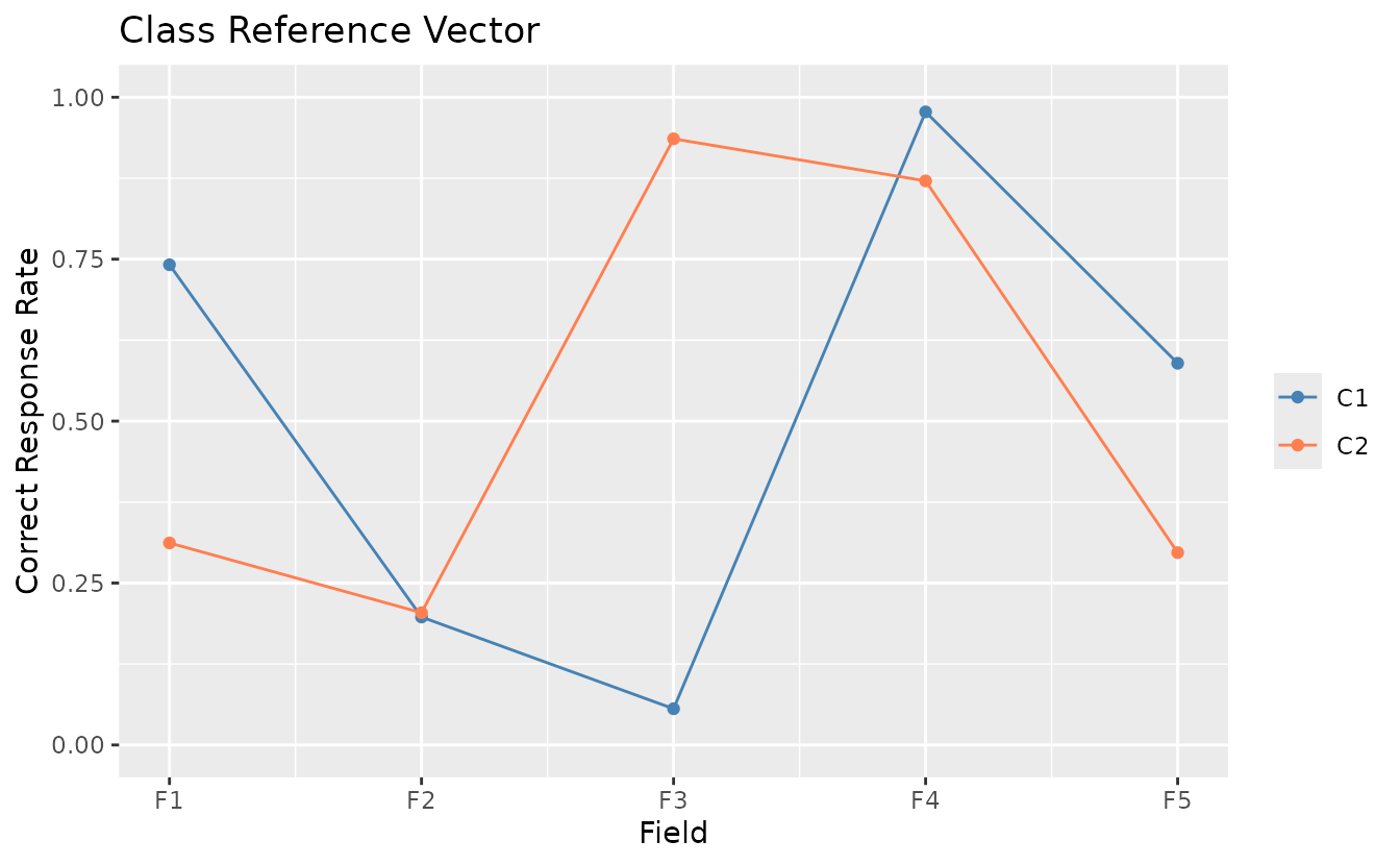
plotCRV_gg — Class Reference Vector
All class profiles in a single plot with one line per class.
plotCRV_gg(result_bic)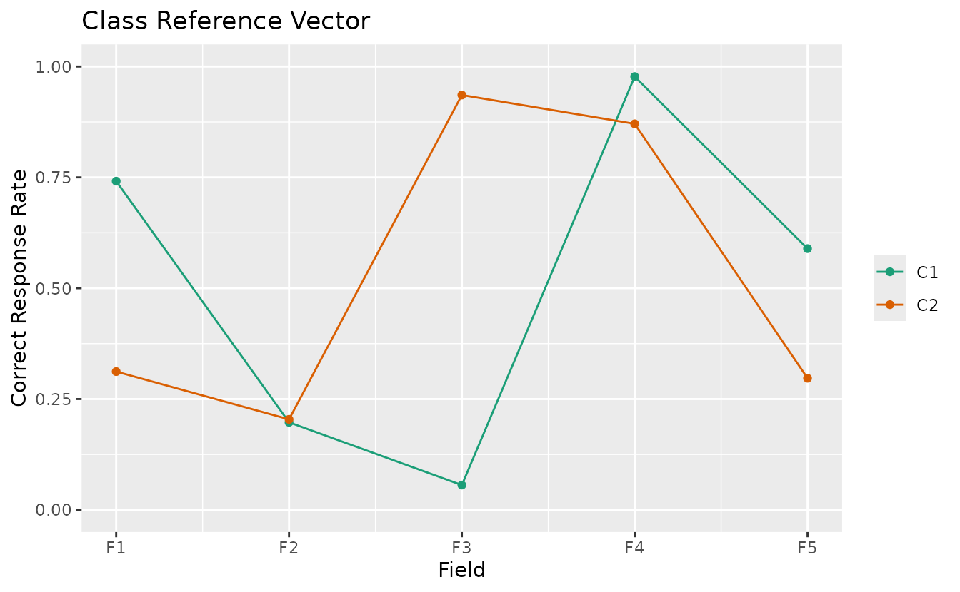
plotRRV_gg — Rank Reference Vector
All rank profiles in a single plot with one line per rank.
plotRRV_gg(result_bic)
plotArray_gg — Array Plot
Visualizes the data matrix as a heatmap showing the block-diagonal structure after biclustering.
plotArray_gg(result_bic)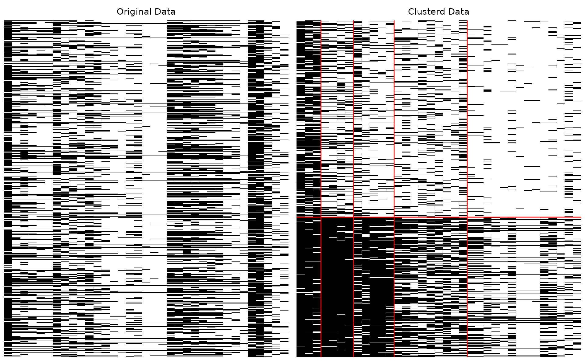
#> TableGrob (1 x 2) "arrange": 2 grobs
#>   z     cells    name           grob
#> 1 1 (1-1,1-1) arrange gtable[layout]
#> 2 2 (1-1,2-2) arrange gtable[layout]
Clustered array only:
plotArray_gg(result_bic, Original = FALSE, Clustered = TRUE)
#> [[1]]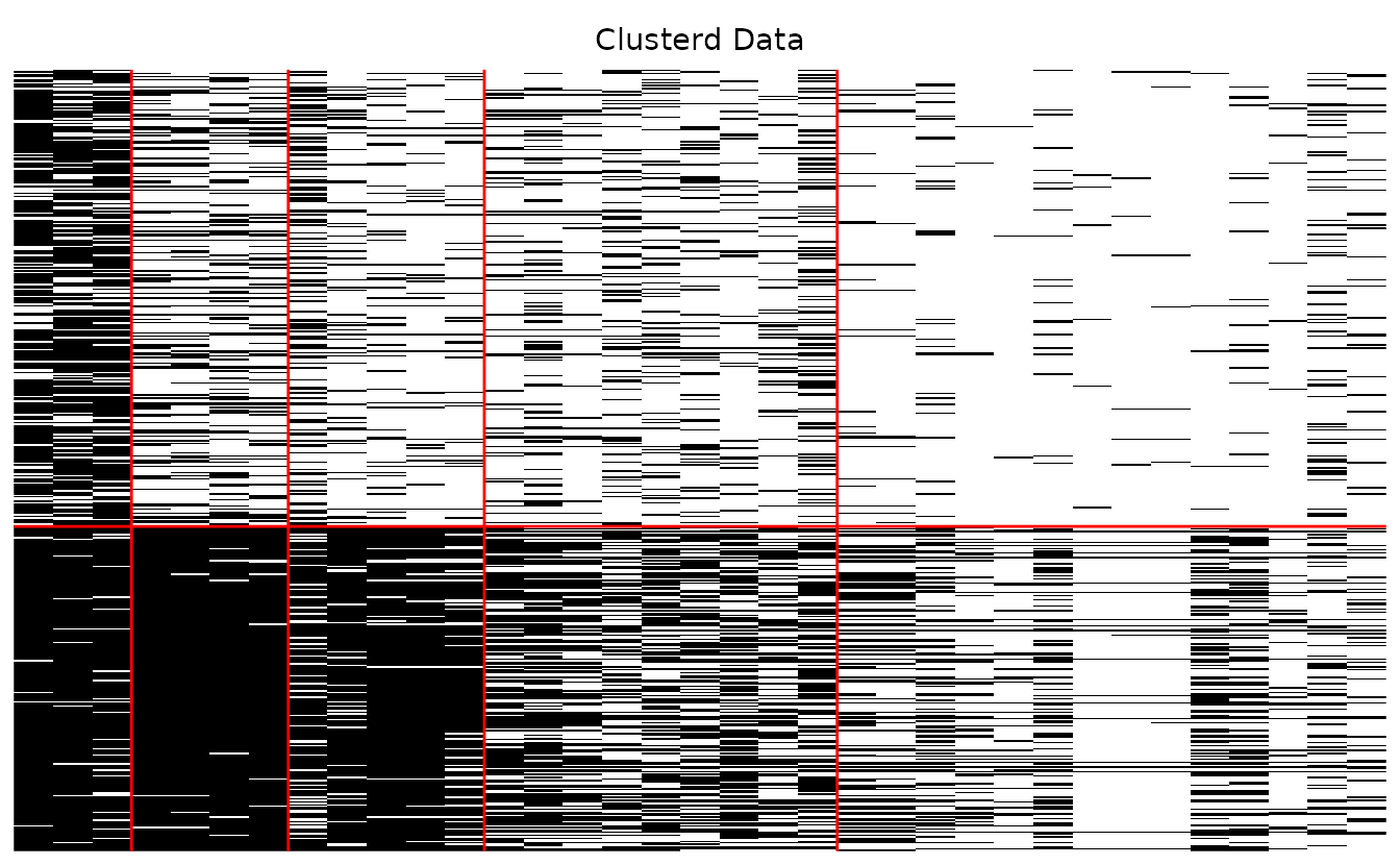
Ordinal Biclustering
Data: J35S500 (35 items, 500 students, 5 categories, 5 fields, 5 classes).
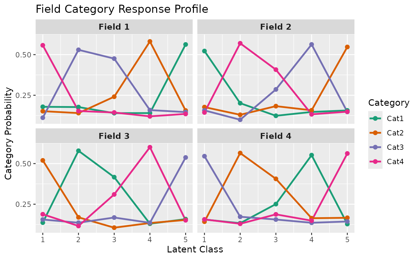
plotFCRP_gg — Field Category Response Profile
Category probability plot with two display styles.
Line style (default):
plotFCRP_gg(result_ord_bic, style = "line")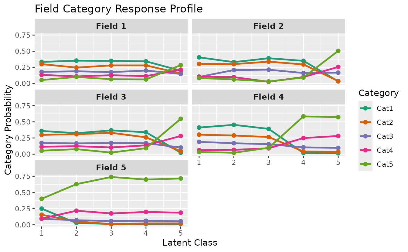
Bar style:
plotFCRP_gg(result_ord_bic, style = "bar")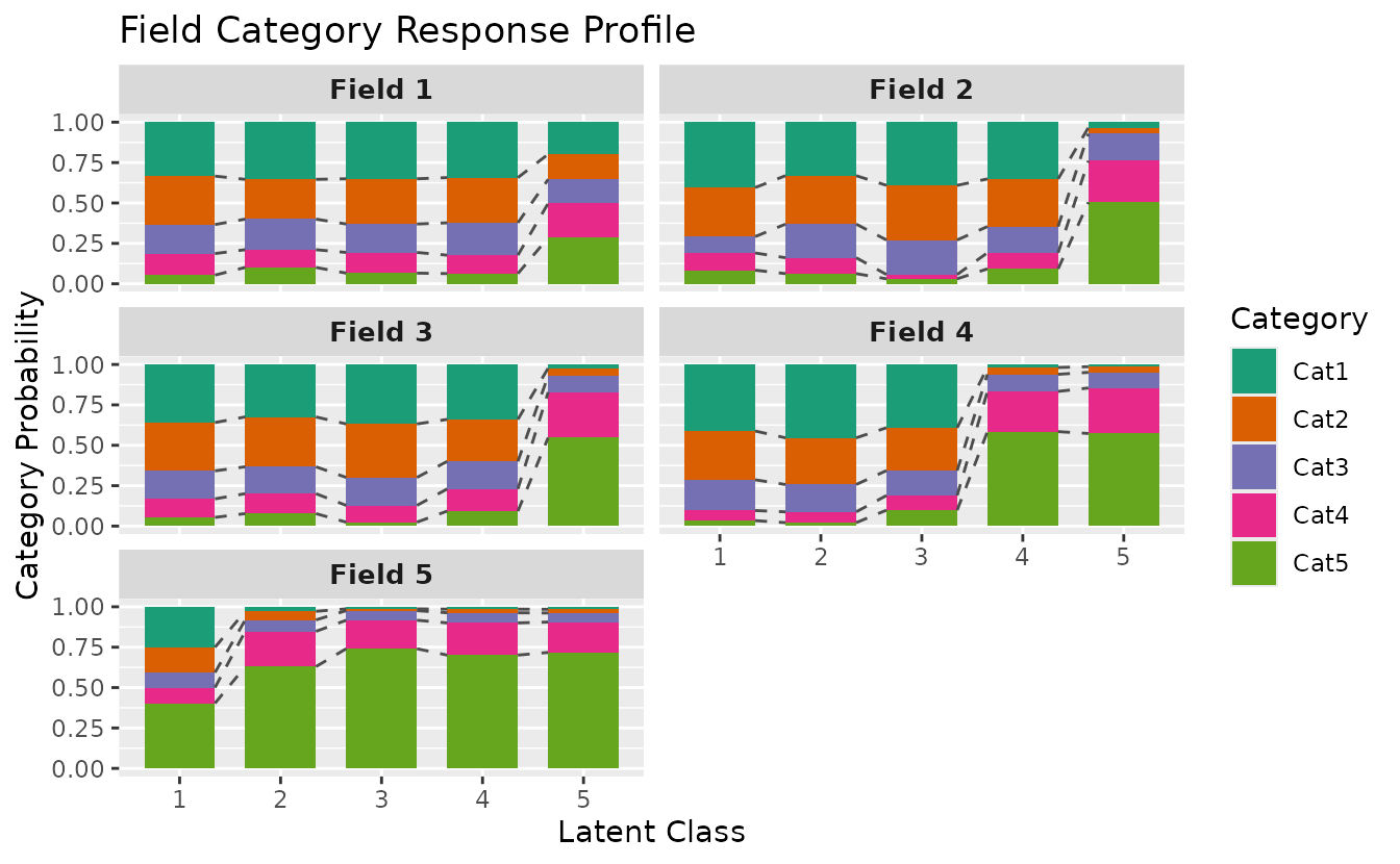
plotFCBR_gg — Field Cumulative Boundary Reference
Boundary probabilities for each field across latent classes. Ordinal Biclustering only.
plotFCBR_gg(result_ord_bic)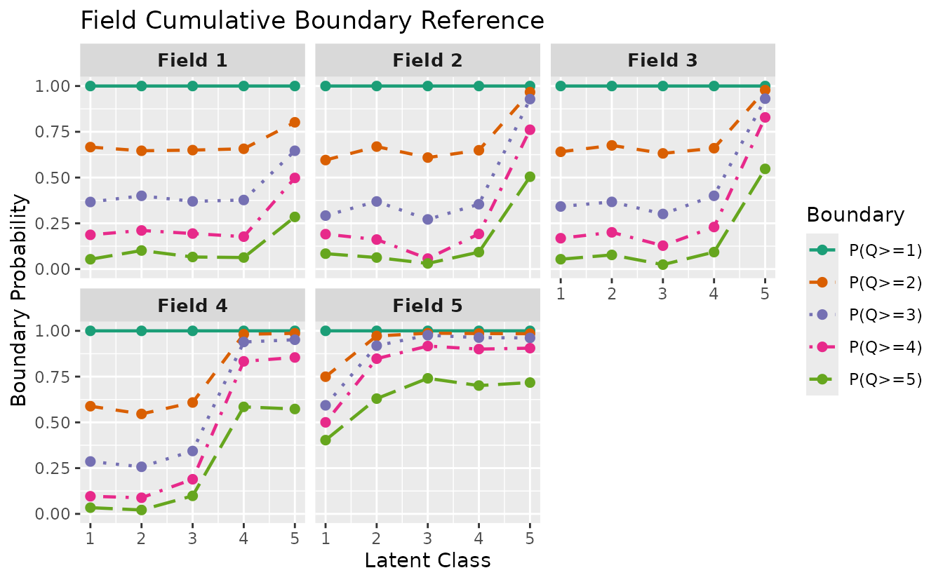
Select specific fields:
plotFCBR_gg(result_ord_bic, fields = 1:3)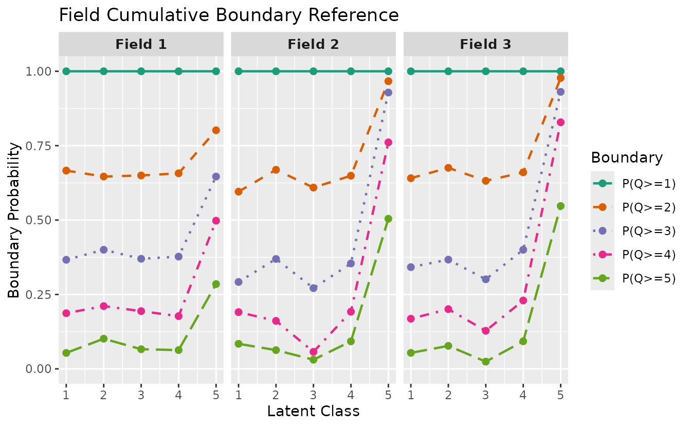
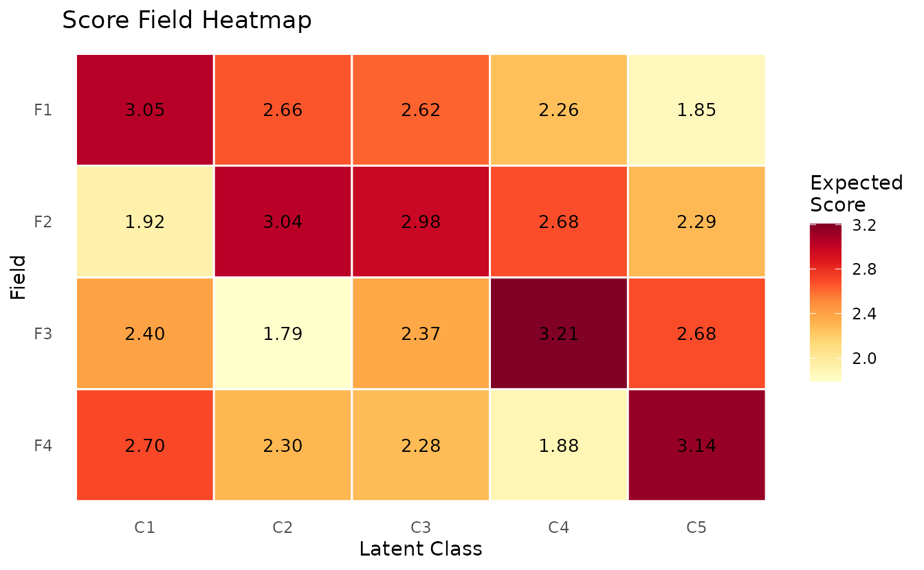
plotScoreField_gg — Expected Score Heatmap
Expected score for each field at each class/rank, displayed as a heatmap.
plotScoreField_gg(result_ord_bic)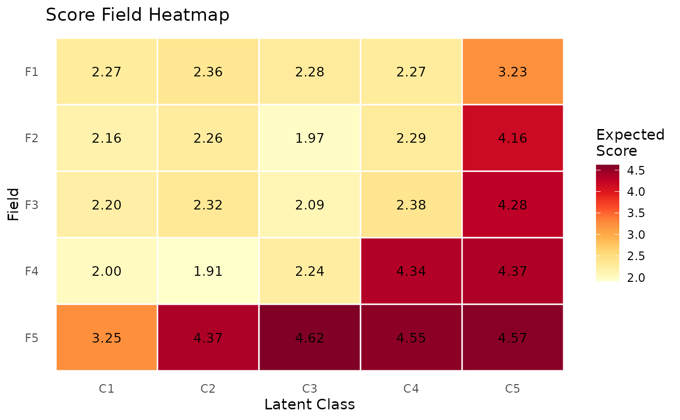
Polytomous stat parameter
plotFRP_gg(), plotCRV_gg(), and
plotRRV_gg() accept a stat parameter for
polytomous data: "mean" (default), "median",
or "mode".
p_mean <- plotFRP_gg(result_ord_bic, stat = "mean") +
  ggplot2::ggtitle("stat = 'mean'")
p_median <- plotFRP_gg(result_ord_bic, stat = "median") +
  ggplot2::ggtitle("stat = 'median'")
p_mode <- plotFRP_gg(result_ord_bic, stat = "mode") +
  ggplot2::ggtitle("stat = 'mode'")
gridExtra::grid.arrange(p_mean, p_median, p_mode, ncol = 2)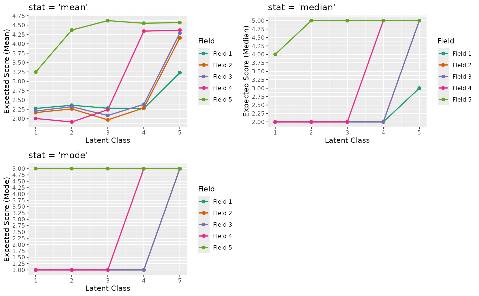
5. LRAordinal / LRArated
Polytomous Latent Rank Analysis with specialized score-level visualizations. Data: J15S3810 (15 items, 3810 students, 4 ranks, ordinal).
plotScoreFreq_gg — Score Frequency Distribution
Density distribution of scores with vertical lines at rank boundary thresholds.
plotScoreFreq_gg(result_lra_ord)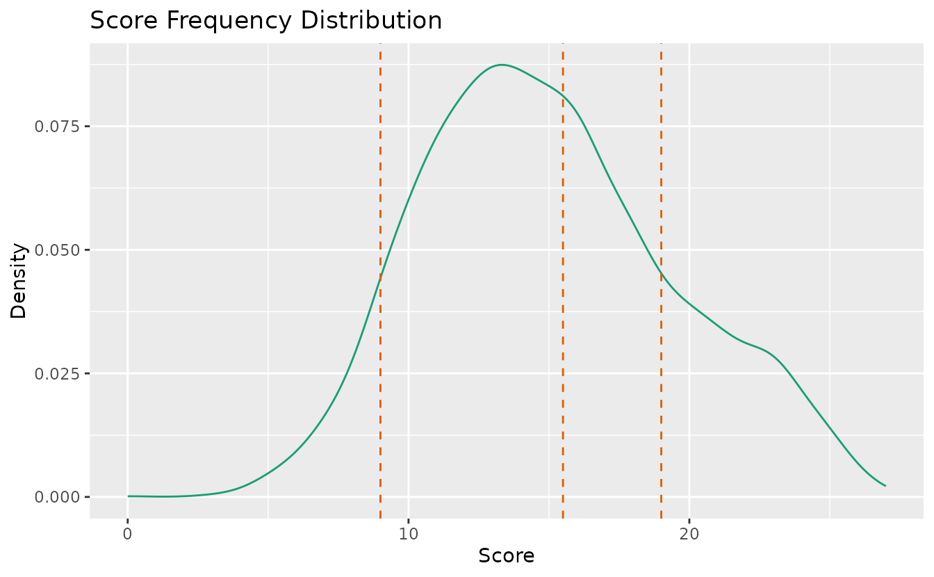
plotScoreRank_gg — Score-Rank Heatmap
Joint distribution of observed scores and estimated ranks. Darker cells indicate higher frequency.
plotScoreRank_gg(result_lra_ord)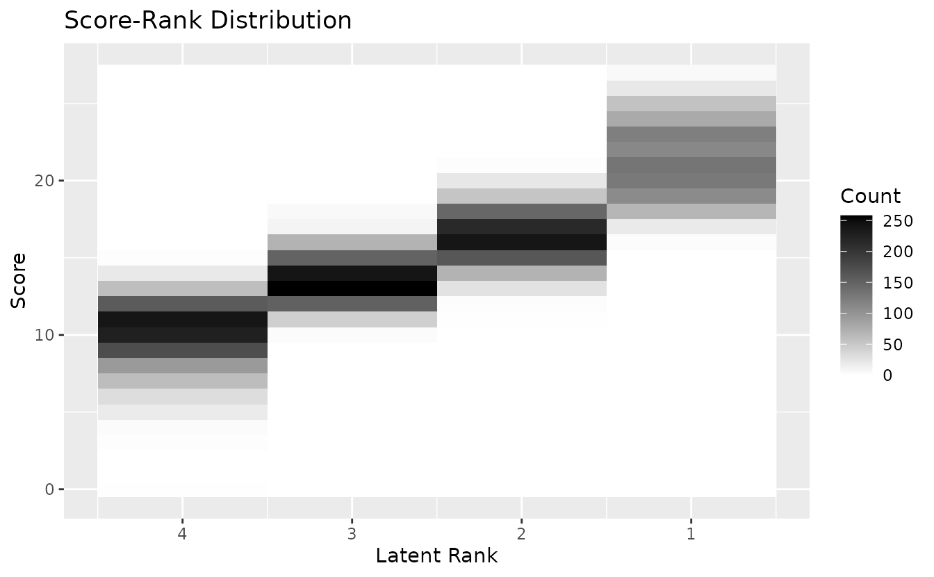
plotICRP_gg — Item Category Reference Profile
Probability of selecting each response category across latent ranks. Probabilities at each rank sum to 1.0.
plotICRP_gg(result_lra_ord, items = 1:4)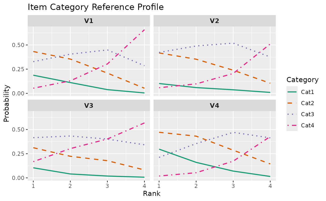
plotICRP_gg(result_lra_ord, items = 5:8)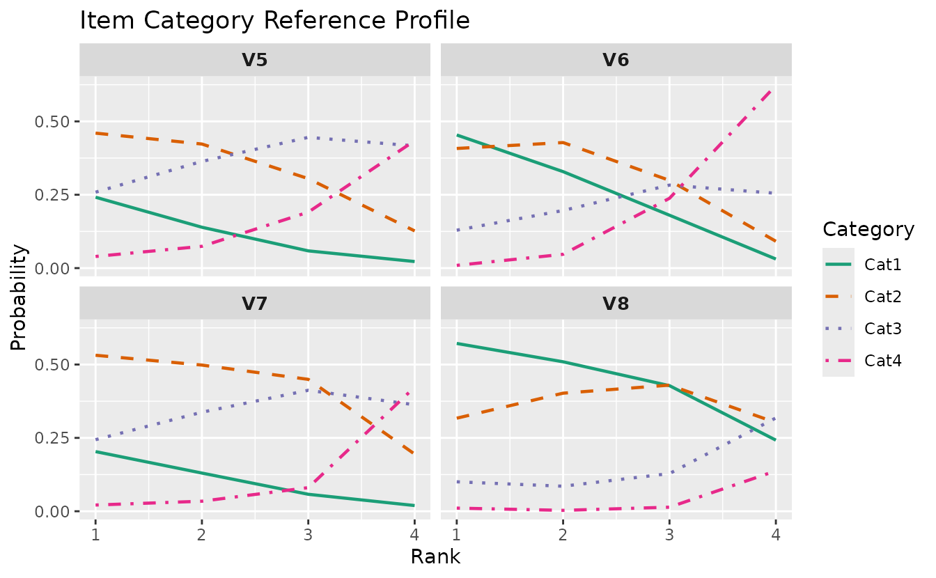
plotICBR_gg — Item Category Boundary Response
Cumulative probability curves for each category boundary. LRAordinal only.
plotICBR_gg(result_lra_ord, items = 1:4)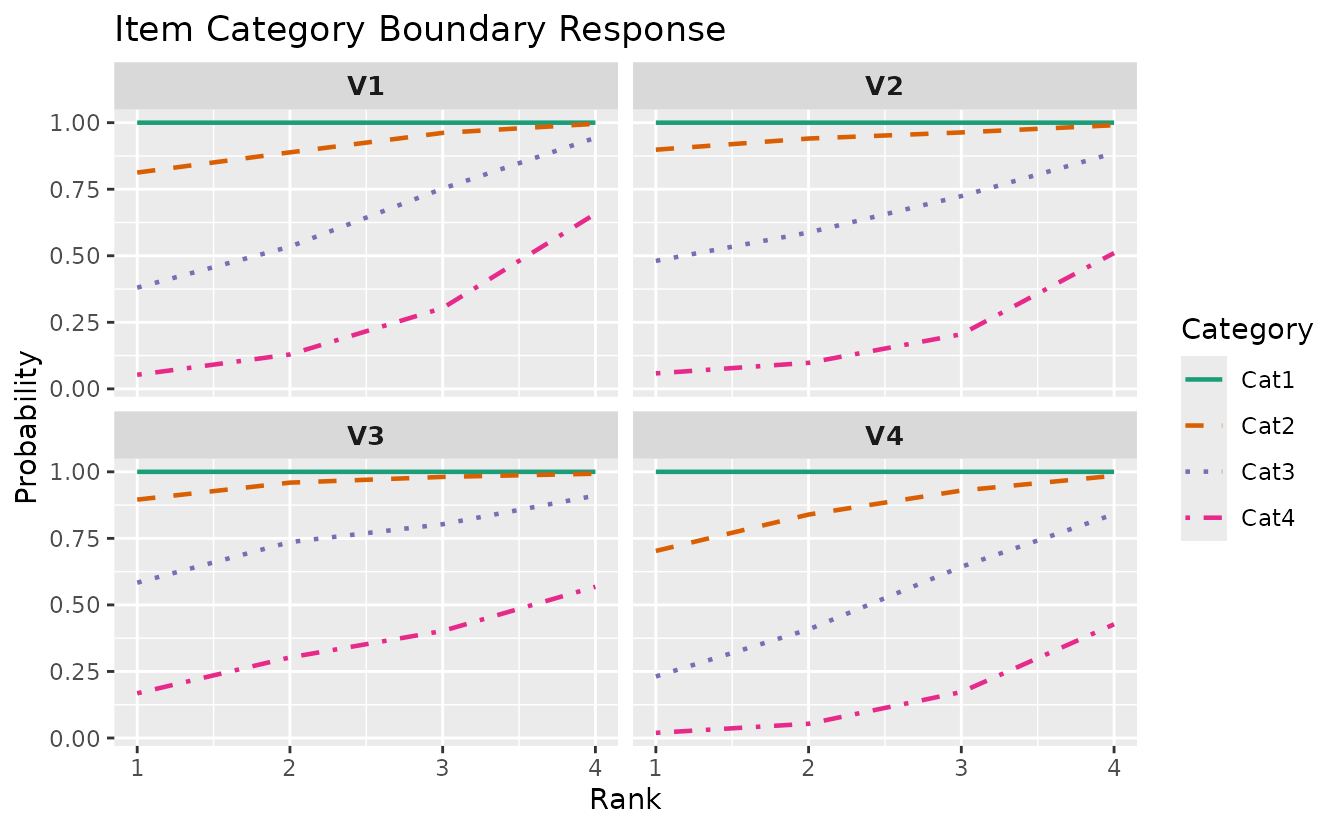
6. Network Models (DAG)
Directed Acyclic Graph and network model visualizations. All four DAG
models are supported by plotGraph_gg(): BNM (items), LDLRA
(items per rank), LDB (fields per rank), and BINET (classes + fields
integrated).
plotGraph_gg — DAG Visualization
BNM (Bayesian Network Model)
The simplest DAG: item-to-item dependency structure. Data: J5S10 (5 items, 10 students).
dag_bnm <- plotGraph_gg(result_bnm)
dag_bnm[[1]]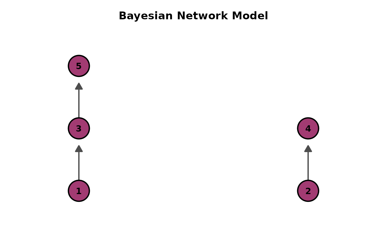
Different layout directions:
bnm_dirs <- lapply(c("BT", "TB", "LR", "RL"), function(d) {
  plotGraph_gg(result_bnm, direction = d, title = paste("BNM -", d))[[1]]
})
gridExtra::grid.arrange(grobs = bnm_dirs, ncol = 2)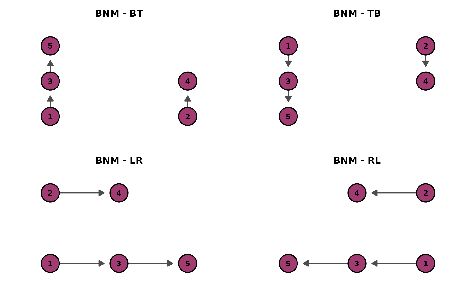
LDLRA (Locally Dependent Latent Rank Analysis)
One DAG per rank, showing how item dependencies change across ranks. Data: J12S5000 (12 items, 5000 students, 3 ranks).
dag_ldlra <- plotGraph_gg(result_ldlra)
combinePlots_gg(dag_ldlra)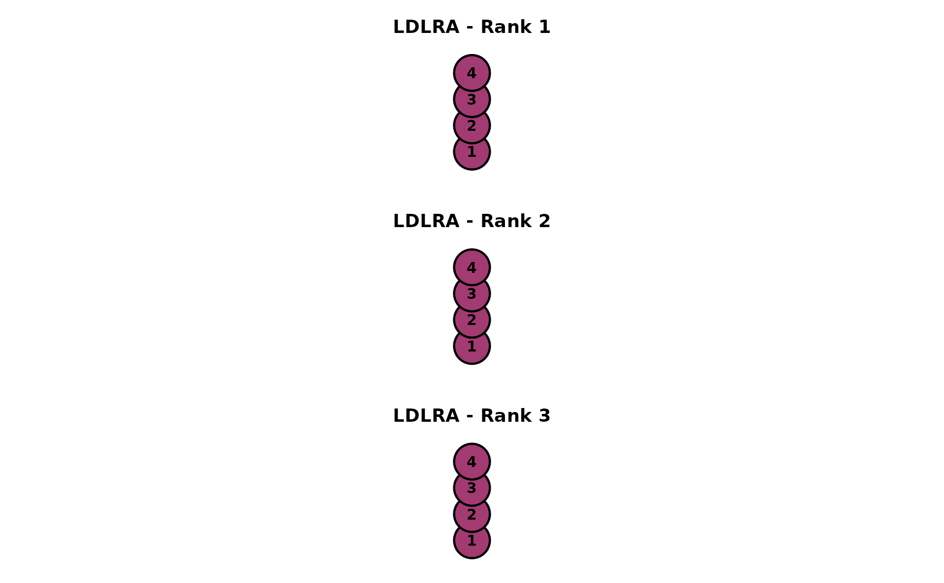
LDB (Locally Dependent Biclustering)
One DAG per rank with field-level nodes (green diamonds). Data: J35S515 (35 items, 515 students, 3 fields, 3 ranks).
dag_ldb <- plotGraph_gg(result_ldb)
combinePlots_gg(dag_ldb)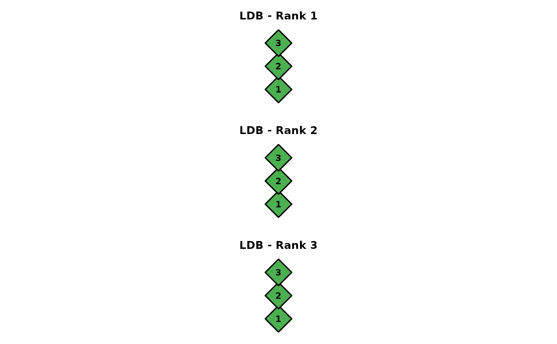
BINET (Bicluster Network Model)
Integrated network with two node types: Class nodes (blue squares) and Field nodes (green diamonds) as intermediates. Data: J35S515 (35 items, 515 students, 3 classes, 3 fields).
dag_binet <- plotGraph_gg(result_binet)
dag_binet[[1]]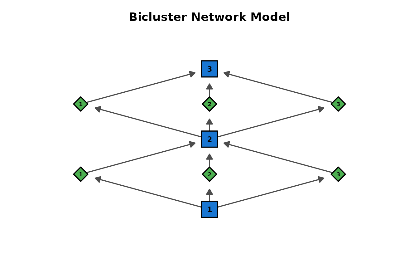
With legend showing node types:
plotGraph_gg(result_binet,
  show_legend = TRUE,
  legend_position = "right", title = "BINET with Legend"
)[[1]]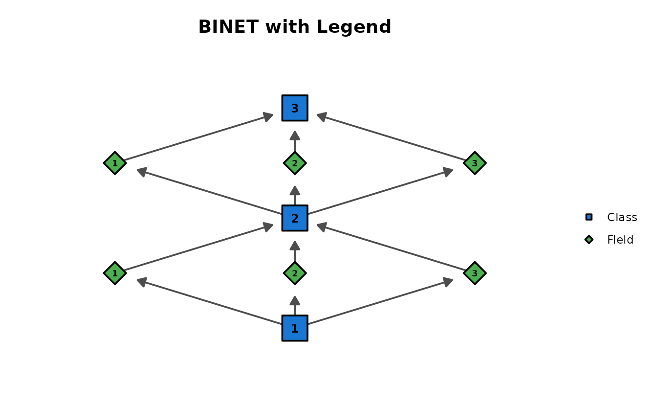
Comparing all four DAG models
p_bnm <- plotGraph_gg(result_bnm, title = "BNM (Items)")[[1]]
p_ldlra <- plotGraph_gg(result_ldlra, title = "LDLRA (Items)")[[1]]
p_ldb <- plotGraph_gg(result_ldb, title = "LDB (Fields)")[[1]]
p_binet <- plotGraph_gg(result_binet,
  title = "BINET (Class+Field)",
  show_legend = TRUE
)[[1]]
gridExtra::grid.arrange(p_bnm, p_ldlra, p_ldb, p_binet, ncol = 2)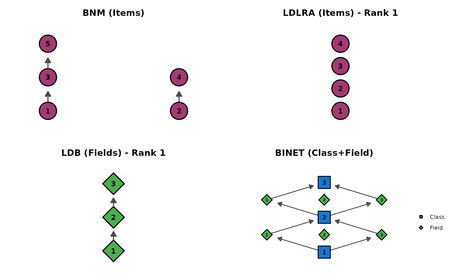
plotFieldPIRP_gg — Field Parent Item Reference Profile
Shows how field performance varies based on parent field scores, for each rank. LDB only. Returns a list of plots (one per rank).
fpirp_plots <- plotFieldPIRP_gg(result_ldb)
combinePlots_gg(fpirp_plots)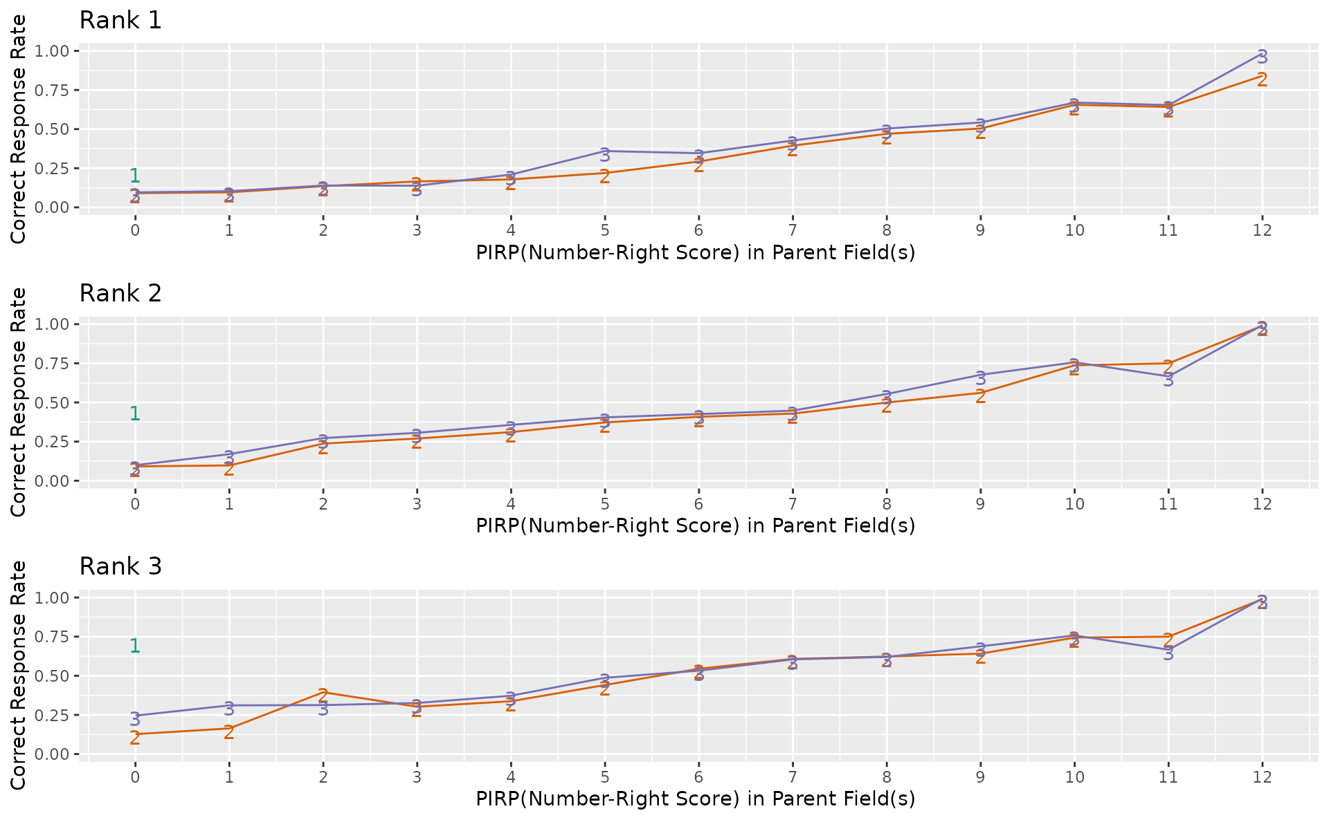
plotLDPSR_gg — Latent Dependence Passing Student Rate
Item-level correct response rate comparing parent and child classes at each DAG edge. BINET only. Returns a list of plots (one per edge).
ldpsr_plots <- plotLDPSR_gg(result_binet)
ldpsr_plots[[1]]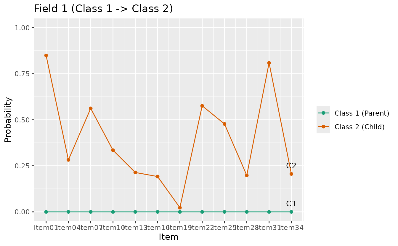
combinePlots_gg(ldpsr_plots, selectPlots = 1:min(6, length(ldpsr_plots)))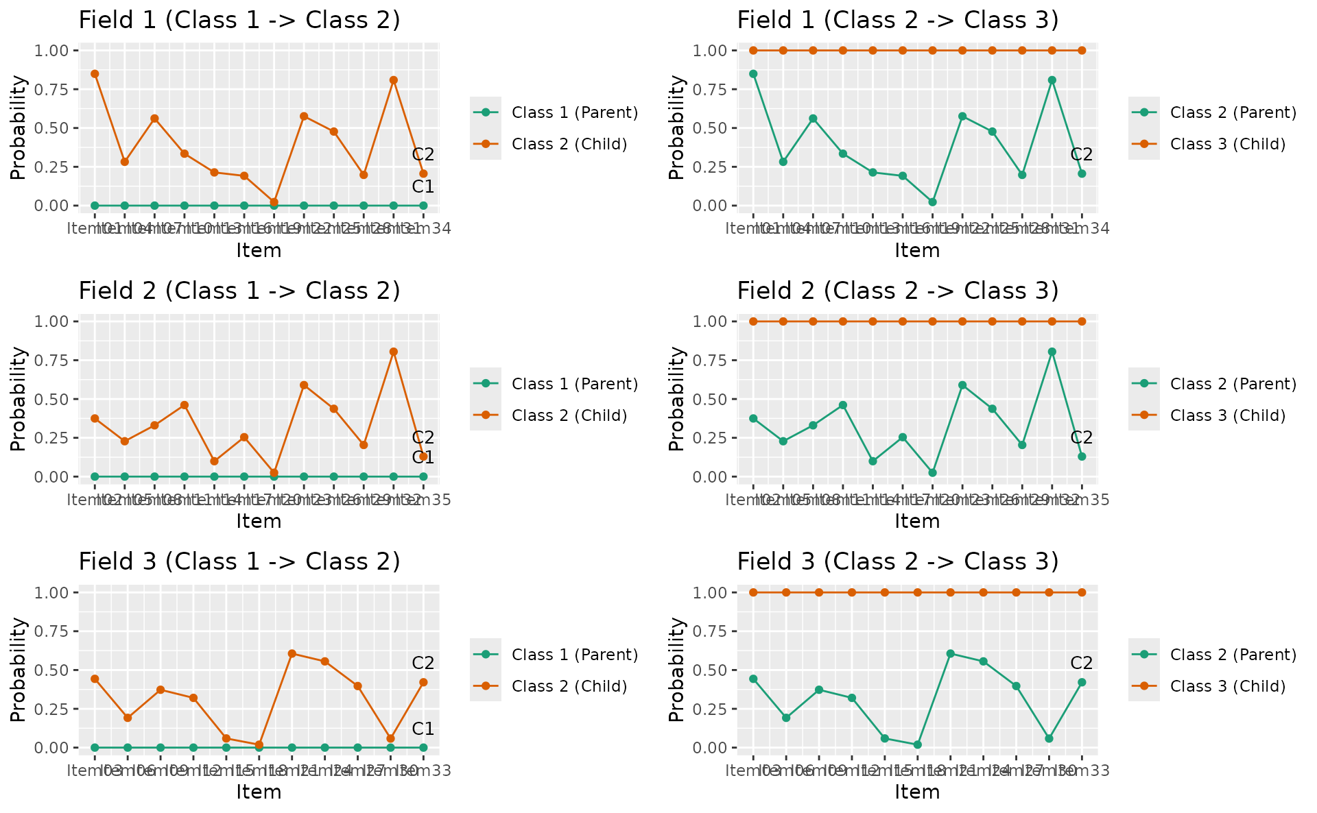
7. Common Options Demo
All plot functions share a consistent set of customization options. Every function returns a ggplot object, so you can add further layers with standard ggplot2 syntax.
| Parameter | Type | Default | Description |
|---|---|---|---|
title |
logical or character | TRUE |
TRUE = auto title, FALSE = hidden,
character = custom |
colors |
character vector | NULL |
NULL = colorblind-friendly palette, or custom
colors |
linetype |
character or numeric | varies |
"solid", "dashed", "dotted",
etc. |
show_legend |
logical | varies | Show or hide the legend |
legend_position |
character | "right" |
"right", "top", "bottom",
"left", "none"
|
title
p1 <- plotICC_overlay_gg(result_irt, items = 1:5, title = TRUE)
p2 <- plotICC_overlay_gg(result_irt, items = 1:5, title = FALSE)
p3 <- plotICC_overlay_gg(result_irt, items = 1:5, title = "My Custom Title")
gridExtra::grid.arrange(p1, p2, p3, ncol = 3)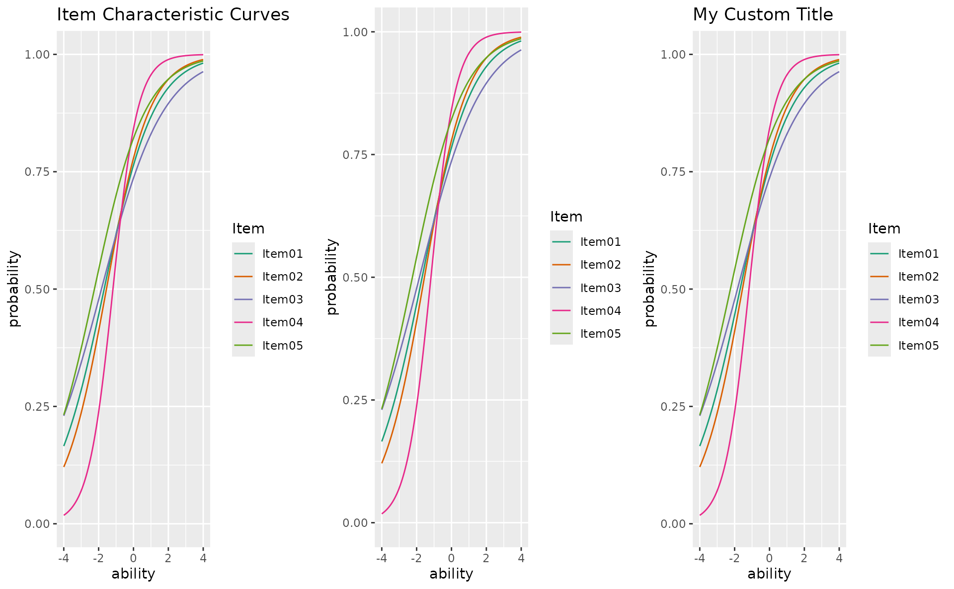
colors
plotICRF_gg(result_grm,
  items = 1,
  colors = c("#D81B60", "#1E88E5", "#FFC107", "#004D40", "#7B1FA2")
)
#> [[1]]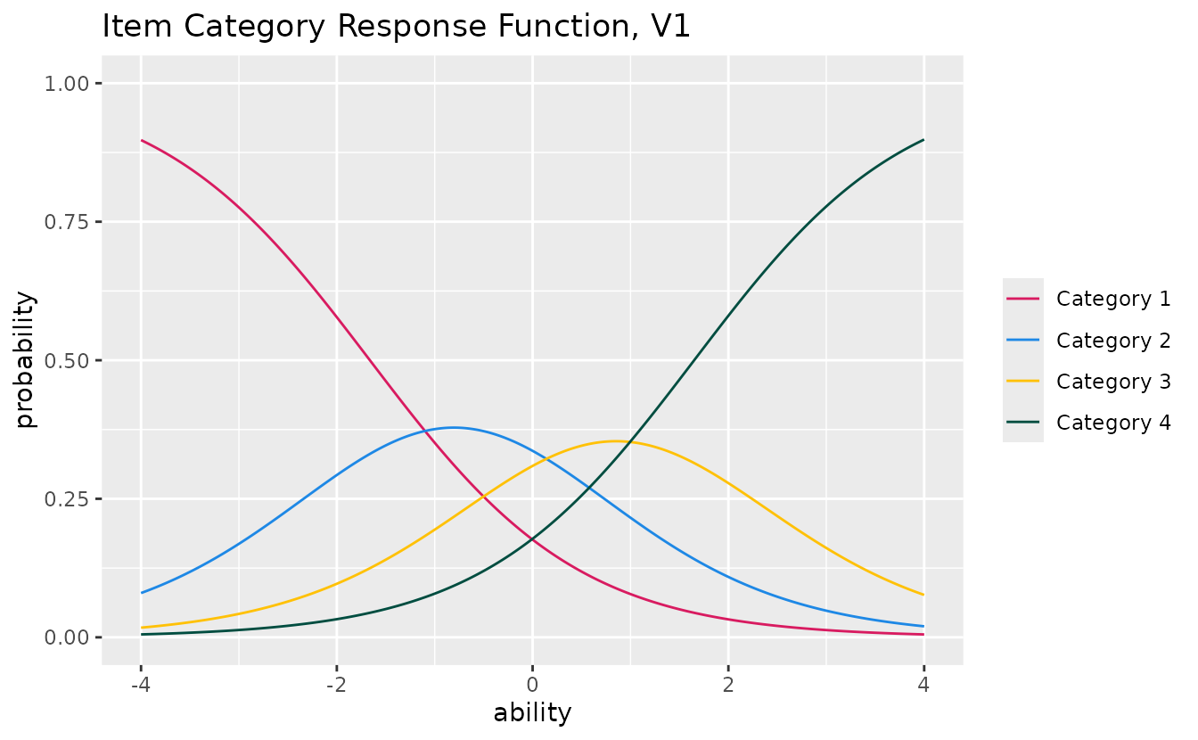
plotCRV_gg(result_bic,
  colors = c(
    "steelblue", "coral", "forestgreen",
    "mediumpurple", "goldenrod", "hotpink"
  )
)
linetype
p1 <- plotTIC_gg(result_irt, linetype = "solid", title = "solid")
p2 <- plotTIC_gg(result_irt, linetype = "dashed", title = "dashed")
p3 <- plotTIC_gg(result_irt, linetype = "dotdash", title = "dotdash")
gridExtra::grid.arrange(p1, p2, p3, ncol = 3)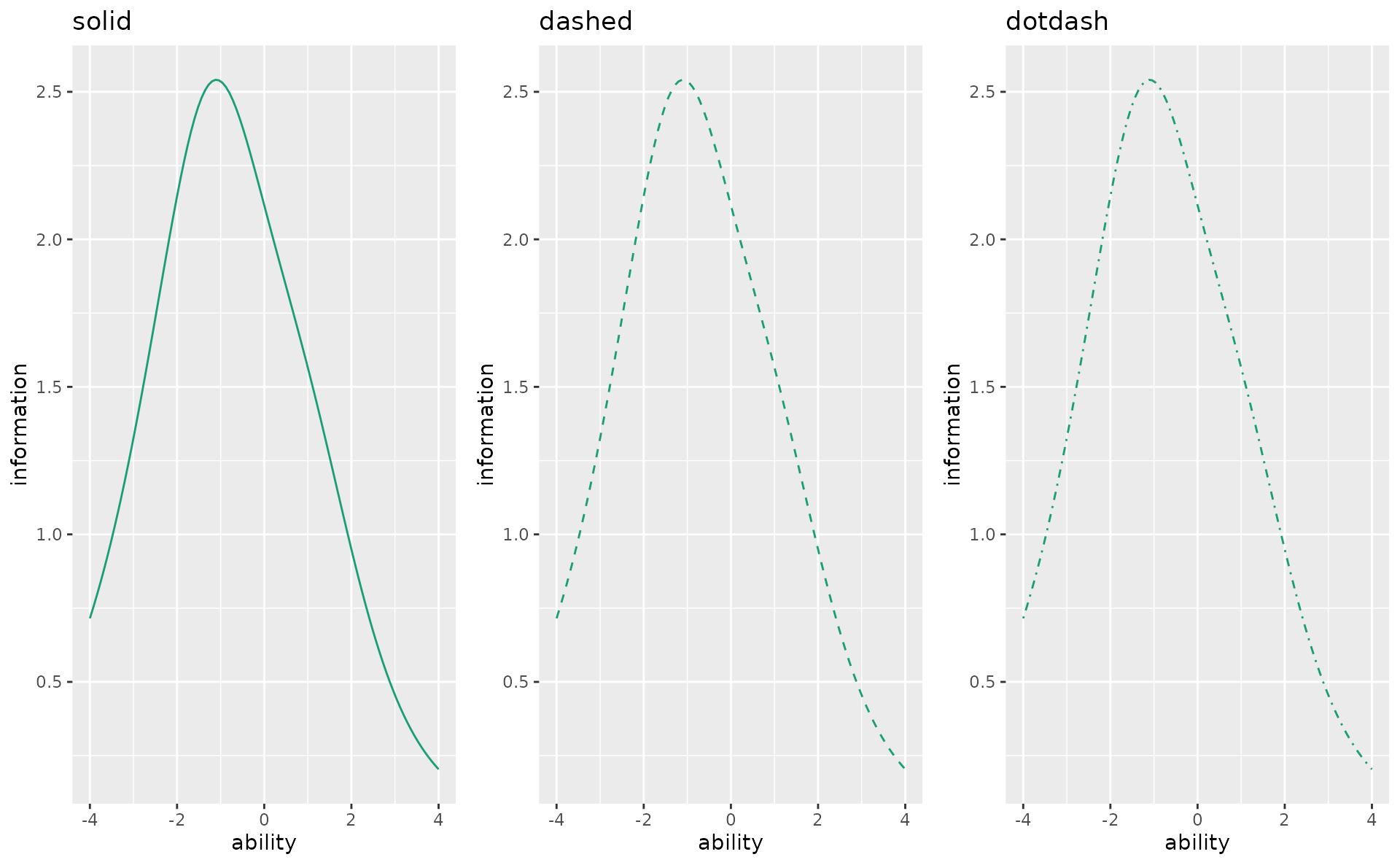
show_legend and legend_position
p1 <- plotICC_overlay_gg(result_irt,
  items = 1:5,
  show_legend = TRUE, legend_position = "right", title = "right"
)
p2 <- plotICC_overlay_gg(result_irt,
  items = 1:5,
  show_legend = TRUE, legend_position = "bottom", title = "bottom"
)
p3 <- plotICC_overlay_gg(result_irt,
  items = 1:5,
  show_legend = TRUE, legend_position = "top", title = "top"
)
p4 <- plotICC_overlay_gg(result_irt,
  items = 1:5,
  show_legend = FALSE, title = "show_legend = FALSE"
)
gridExtra::grid.arrange(p1, p2, p3, p4, ncol = 2)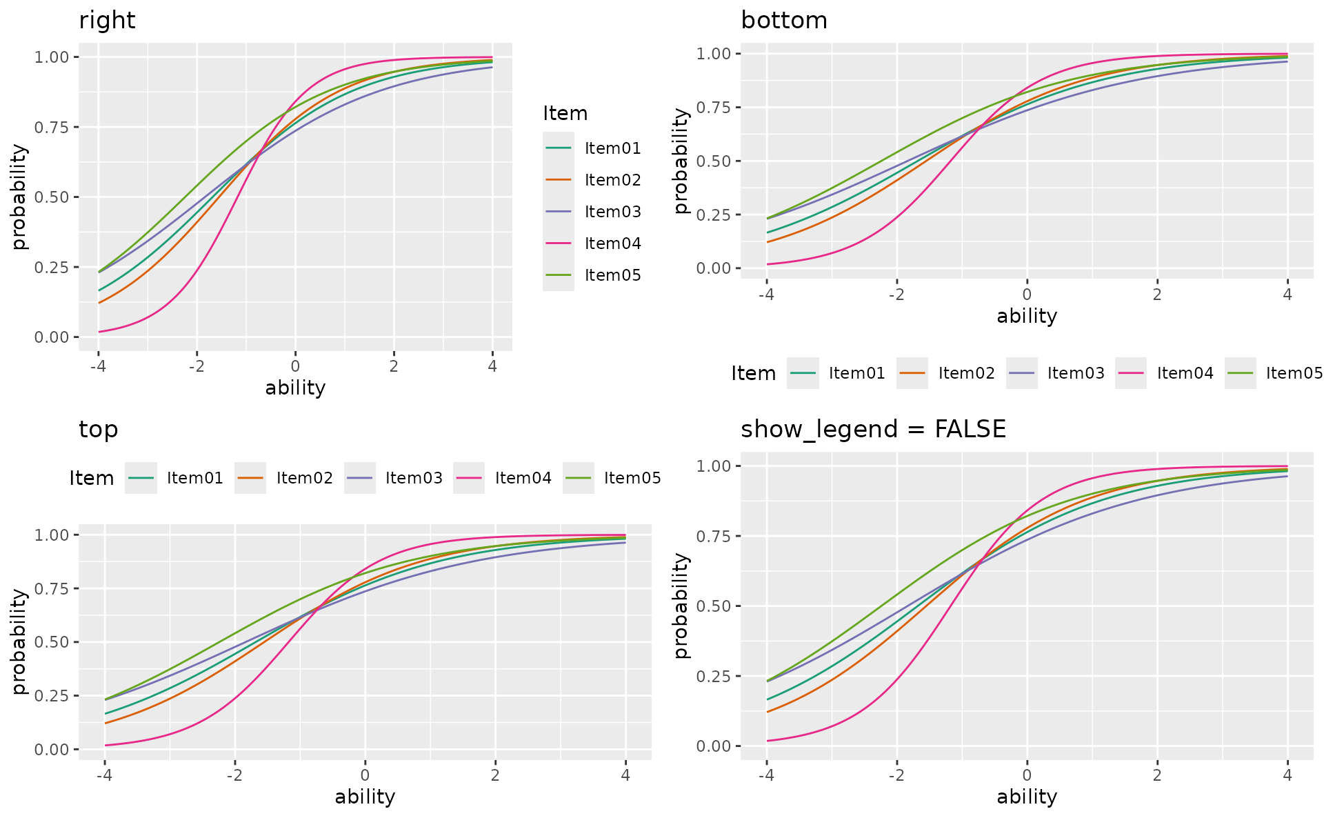
Combining options
plotICRF_gg(result_grm,
  items = 1,
  title = "Fully Customized ICRF",
  colors = c("#E41A1C", "#377EB8", "#4DAF4A", "#984EA3", "#FF7F00"),
  linetype = "solid",
  show_legend = TRUE,
  legend_position = "bottom"
)
#> [[1]]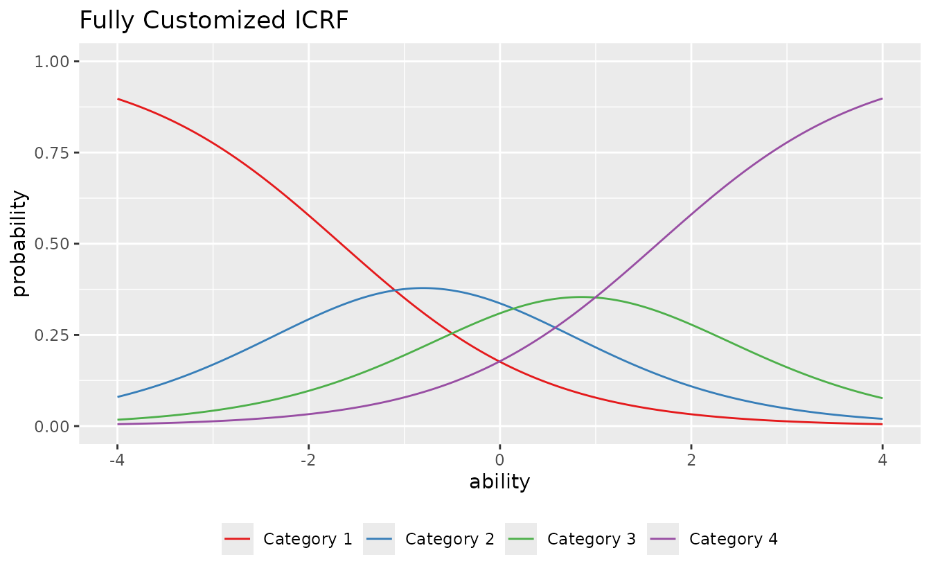
Post-hoc ggplot2 customization
Since all functions return ggplot objects, you can add any ggplot2 layer:
plotTIC_gg(result_irt) +
  ggplot2::theme_minimal() +
  ggplot2::labs(
    subtitle = "Custom subtitle via ggplot2",
    caption = "Generated with ggExametrika"
  )