準備

パッケージの読み込み

library(brms)

## Loading required package: Rcpp

## Loading required package: ggplot2

## Loading 'brms' package (version 2.7.0). Useful instructions
## can be found by typing help('brms'). A more detailed introduction
## to the package is available through vignette('brms_overview').
## Run theme_set(theme_default()) to use the default bayesplot theme.

library(tidyverse)

## ─ Attaching packages ────────────────────────────────── tidyverse 1.2.1 ─

## ✔ tibble  2.0.1       ✔ purrr   0.3.1  
## ✔ tidyr   0.8.3       ✔ dplyr   0.8.0.1
## ✔ readr   1.3.1       ✔ stringr 1.4.0  
## ✔ tibble  2.0.1       ✔ forcats 0.4.0

## ─ Conflicts ──────────────────────────────────── tidyverse_conflicts() ─
## ✖ dplyr::filter() masks stats::filter()
## ✖ dplyr::lag()    masks stats::lag()

データ

今回使うデータははRの持っているサンプルデータです。車のメーカ(manufacture)，モデル(model)，排気量(displ)，製造年(year)，気筒数(cyl)，オートマ・マニュアルの別(trans), 駆動輪(drv)，市街地での燃費(cty)，高速道路での燃費(hwy)などからなるデータセットです。

data(mpg)
# 少しみてみる
head(mpg)

manufacturer	model	displ	year	cyl	trans	drv	cty	hwy	fl	class
audi	a4	1.8	1999	4	auto(l5)	f	18	29	p	compact
audi	a4	1.8	1999	4	manual(m5)	f	21	29	p	compact
audi	a4	2.0	2008	4	manual(m6)	f	20	31	p	compact
audi	a4	2.0	2008	4	auto(av)	f	21	30	p	compact
audi	a4	2.8	1999	6	auto(l5)	f	16	26	p	compact
audi	a4	2.8	1999	6	manual(m5)	f	18	26	p	compact

可視化してみましょう

排気量と市街地での燃費の関係をグラフにします。

g <- ggplot(mpg,aes(x=displ,y=cty))+geom_point()
plot(g)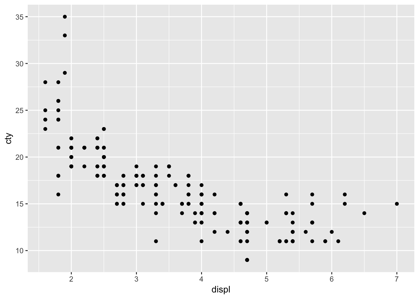

回帰線を追加します。

g <- g + geom_smooth(method='lm')
plot(g)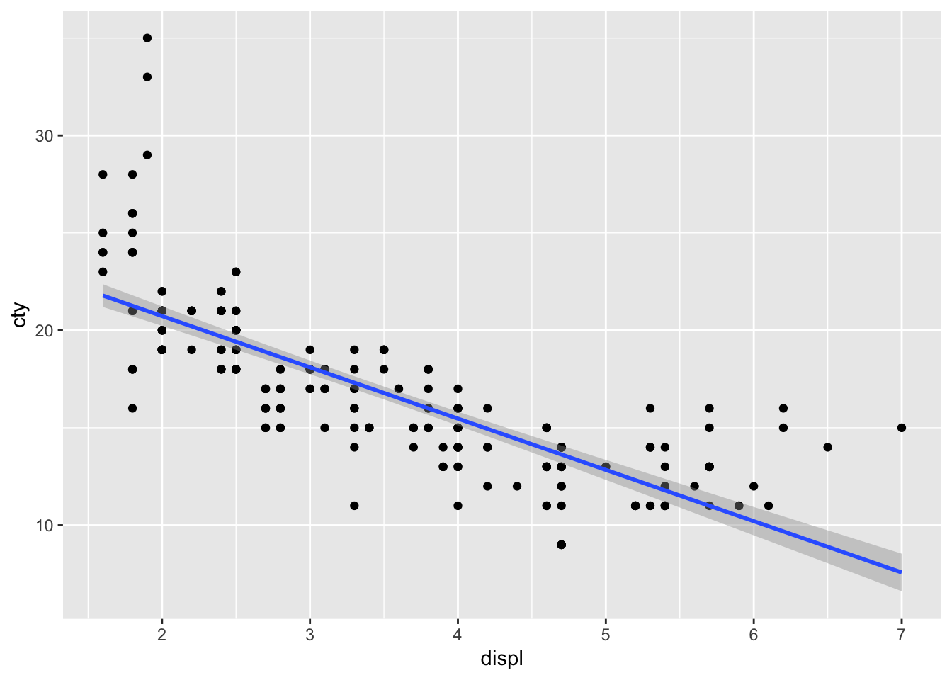

最尤法による回帰

summary(lm(cty~displ,data=mpg))

## 
## Call:
## lm(formula = cty ~ displ, data = mpg)
## 
## Residuals:
##     Min      1Q  Median      3Q     Max 
## -6.3109 -1.4695 -0.2566  1.1087 14.0064 
## 
## Coefficients:
##             Estimate Std. Error t value Pr(>|t|)    
## (Intercept)  25.9915     0.4821   53.91   <2e-16 ***
## displ        -2.6305     0.1302  -20.20   <2e-16 ***
## ---
## Signif. codes:  0 '***' 0.001 '**' 0.01 '*' 0.05 '.' 0.1 ' ' 1
## 
## Residual standard error: 2.567 on 232 degrees of freedom
## Multiple R-squared:  0.6376, Adjusted R-squared:  0.6361 
## F-statistic: 408.2 on 1 and 232 DF,  p-value: < 2.2e-16

回帰線のベイズ推定

result.brm <- brm(cty~displ,data=mpg)

## Compiling the C++ model

## Start sampling

## 
## SAMPLING FOR MODEL '7e5af2e7cd64c4d926e4c21aec634789' NOW (CHAIN 1).
## Chain 1: 
## Chain 1: Gradient evaluation took 4.2e-05 seconds
## Chain 1: 1000 transitions using 10 leapfrog steps per transition would take 0.42 seconds.
## Chain 1: Adjust your expectations accordingly!
## Chain 1: 
## Chain 1: 
## Chain 1: Iteration:    1 / 2000 [  0%]  (Warmup)
## Chain 1: Iteration:  200 / 2000 [ 10%]  (Warmup)
## Chain 1: Iteration:  400 / 2000 [ 20%]  (Warmup)
## Chain 1: Iteration:  600 / 2000 [ 30%]  (Warmup)
## Chain 1: Iteration:  800 / 2000 [ 40%]  (Warmup)
## Chain 1: Iteration: 1000 / 2000 [ 50%]  (Warmup)
## Chain 1: Iteration: 1001 / 2000 [ 50%]  (Sampling)
## Chain 1: Iteration: 1200 / 2000 [ 60%]  (Sampling)
## Chain 1: Iteration: 1400 / 2000 [ 70%]  (Sampling)
## Chain 1: Iteration: 1600 / 2000 [ 80%]  (Sampling)
## Chain 1: Iteration: 1800 / 2000 [ 90%]  (Sampling)
## Chain 1: Iteration: 2000 / 2000 [100%]  (Sampling)
## Chain 1: 
## Chain 1:  Elapsed Time: 0.057783 seconds (Warm-up)
## Chain 1:                0.047749 seconds (Sampling)
## Chain 1:                0.105532 seconds (Total)
## Chain 1: 
## 
## SAMPLING FOR MODEL '7e5af2e7cd64c4d926e4c21aec634789' NOW (CHAIN 2).
## Chain 2: 
## Chain 2: Gradient evaluation took 1.5e-05 seconds
## Chain 2: 1000 transitions using 10 leapfrog steps per transition would take 0.15 seconds.
## Chain 2: Adjust your expectations accordingly!
## Chain 2: 
## Chain 2: 
## Chain 2: Iteration:    1 / 2000 [  0%]  (Warmup)
## Chain 2: Iteration:  200 / 2000 [ 10%]  (Warmup)
## Chain 2: Iteration:  400 / 2000 [ 20%]  (Warmup)
## Chain 2: Iteration:  600 / 2000 [ 30%]  (Warmup)
## Chain 2: Iteration:  800 / 2000 [ 40%]  (Warmup)
## Chain 2: Iteration: 1000 / 2000 [ 50%]  (Warmup)
## Chain 2: Iteration: 1001 / 2000 [ 50%]  (Sampling)
## Chain 2: Iteration: 1200 / 2000 [ 60%]  (Sampling)
## Chain 2: Iteration: 1400 / 2000 [ 70%]  (Sampling)
## Chain 2: Iteration: 1600 / 2000 [ 80%]  (Sampling)
## Chain 2: Iteration: 1800 / 2000 [ 90%]  (Sampling)
## Chain 2: Iteration: 2000 / 2000 [100%]  (Sampling)
## Chain 2: 
## Chain 2:  Elapsed Time: 0.057174 seconds (Warm-up)
## Chain 2:                0.092456 seconds (Sampling)
## Chain 2:                0.14963 seconds (Total)
## Chain 2: 
## 
## SAMPLING FOR MODEL '7e5af2e7cd64c4d926e4c21aec634789' NOW (CHAIN 3).
## Chain 3: 
## Chain 3: Gradient evaluation took 1.3e-05 seconds
## Chain 3: 1000 transitions using 10 leapfrog steps per transition would take 0.13 seconds.
## Chain 3: Adjust your expectations accordingly!
## Chain 3: 
## Chain 3: 
## Chain 3: Iteration:    1 / 2000 [  0%]  (Warmup)
## Chain 3: Iteration:  200 / 2000 [ 10%]  (Warmup)
## Chain 3: Iteration:  400 / 2000 [ 20%]  (Warmup)
## Chain 3: Iteration:  600 / 2000 [ 30%]  (Warmup)
## Chain 3: Iteration:  800 / 2000 [ 40%]  (Warmup)
## Chain 3: Iteration: 1000 / 2000 [ 50%]  (Warmup)
## Chain 3: Iteration: 1001 / 2000 [ 50%]  (Sampling)
## Chain 3: Iteration: 1200 / 2000 [ 60%]  (Sampling)
## Chain 3: Iteration: 1400 / 2000 [ 70%]  (Sampling)
## Chain 3: Iteration: 1600 / 2000 [ 80%]  (Sampling)
## Chain 3: Iteration: 1800 / 2000 [ 90%]  (Sampling)
## Chain 3: Iteration: 2000 / 2000 [100%]  (Sampling)
## Chain 3: 
## Chain 3:  Elapsed Time: 0.056806 seconds (Warm-up)
## Chain 3:                0.090612 seconds (Sampling)
## Chain 3:                0.147418 seconds (Total)
## Chain 3: 
## 
## SAMPLING FOR MODEL '7e5af2e7cd64c4d926e4c21aec634789' NOW (CHAIN 4).
## Chain 4: 
## Chain 4: Gradient evaluation took 1.3e-05 seconds
## Chain 4: 1000 transitions using 10 leapfrog steps per transition would take 0.13 seconds.
## Chain 4: Adjust your expectations accordingly!
## Chain 4: 
## Chain 4: 
## Chain 4: Iteration:    1 / 2000 [  0%]  (Warmup)
## Chain 4: Iteration:  200 / 2000 [ 10%]  (Warmup)
## Chain 4: Iteration:  400 / 2000 [ 20%]  (Warmup)
## Chain 4: Iteration:  600 / 2000 [ 30%]  (Warmup)
## Chain 4: Iteration:  800 / 2000 [ 40%]  (Warmup)
## Chain 4: Iteration: 1000 / 2000 [ 50%]  (Warmup)
## Chain 4: Iteration: 1001 / 2000 [ 50%]  (Sampling)
## Chain 4: Iteration: 1200 / 2000 [ 60%]  (Sampling)
## Chain 4: Iteration: 1400 / 2000 [ 70%]  (Sampling)
## Chain 4: Iteration: 1600 / 2000 [ 80%]  (Sampling)
## Chain 4: Iteration: 1800 / 2000 [ 90%]  (Sampling)
## Chain 4: Iteration: 2000 / 2000 [100%]  (Sampling)
## Chain 4: 
## Chain 4:  Elapsed Time: 0.058578 seconds (Warm-up)
## Chain 4:                0.051714 seconds (Sampling)
## Chain 4:                0.110292 seconds (Total)
## Chain 4:

result.brm

##  Family: gaussian 
##   Links: mu = identity; sigma = identity 
## Formula: cty ~ displ 
##    Data: mpg (Number of observations: 234) 
## Samples: 4 chains, each with iter = 2000; warmup = 1000; thin = 1;
##          total post-warmup samples = 4000
## 
## Population-Level Effects: 
##           Estimate Est.Error l-95% CI u-95% CI Eff.Sample Rhat
## Intercept    25.99      0.48    25.07    26.93       4391 1.00
## displ        -2.63      0.13    -2.89    -2.38       4268 1.00
## 
## Family Specific Parameters: 
##       Estimate Est.Error l-95% CI u-95% CI Eff.Sample Rhat
## sigma     2.58      0.12     2.36     2.82       4423 1.00
## 
## Samples were drawn using sampling(NUTS). For each parameter, Eff.Sample 
## is a crude measure of effective sample size, and Rhat is the potential 
## scale reduction factor on split chains (at convergence, Rhat = 1).

結果のプロット

事後分布とトレースプロット

plot(result.brm)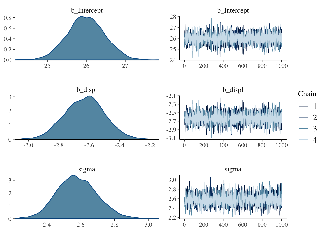

MCMCサンプルをみてみる

# 取り出し -> データフレーム型へ　-> 頭の10行だけ表示
rstan::extract(result.brm$fit) %>% data.frame %>% head(10)

b_Intercept	b	sigma	lp__
25.11060	-2.370101	2.674755	-558.9614
26.04493	-2.606203	2.549161	-557.0499
26.20681	-2.735127	2.681749	-557.8145
26.39549	-2.743991	2.490659	-557.2777
25.93521	-2.619741	2.653101	-556.9761
26.67031	-2.762573	2.596664	-558.0733
25.65094	-2.549842	2.743078	-557.9566
25.35317	-2.505538	2.422382	-558.7917
26.29992	-2.739840	2.645074	-557.3383
26.70885	-2.785200	2.497674	-558.1914

回帰線のグラフ

plot(marginal_effects(result.brm))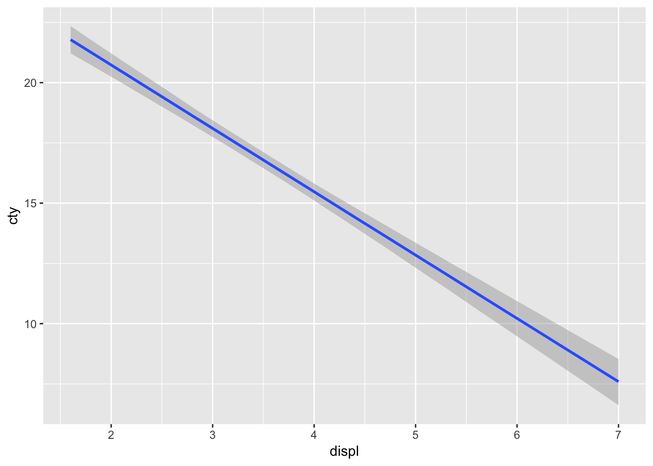

事後予測分布

pp_check(result.brm)

## Using 10 posterior samples for ppc type 'dens_overlay' by default.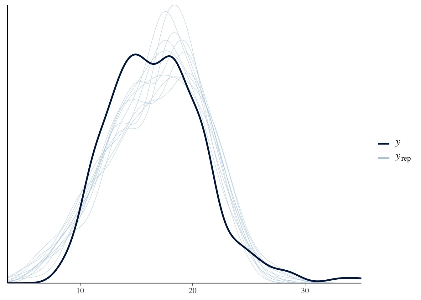

事後予測分布

predict(result.brm) %>% head(10)

##       Estimate Est.Error     Q2.5    Q97.5
##  [1,] 21.31048  2.599970 16.09270 26.31486
##  [2,] 21.31205  2.573370 16.27210 26.22410
##  [3,] 20.68270  2.646399 15.46692 26.10699
##  [4,] 20.80638  2.563281 15.68658 25.83451
##  [5,] 18.63636  2.603001 13.50303 23.74901
##  [6,] 18.66532  2.569043 13.56937 23.55285
##  [7,] 17.93478  2.642655 12.84637 23.23644
##  [8,] 21.21270  2.583297 16.13018 26.31577
##  [9,] 21.25033  2.622059 16.03771 26.29970
## [10,] 20.74153  2.587537 15.60967 25.75037

分析に使ったstanコードも出力できる

result.brm$model

## // generated with brms 2.7.0
## functions { 
## } 
## data { 
##   int<lower=1> N;  // total number of observations 
##   vector[N] Y;  // response variable 
##   int<lower=1> K;  // number of population-level effects 
##   matrix[N, K] X;  // population-level design matrix 
##   int prior_only;  // should the likelihood be ignored? 
## } 
## transformed data { 
##   int Kc = K - 1; 
##   matrix[N, K - 1] Xc;  // centered version of X 
##   vector[K - 1] means_X;  // column means of X before centering 
##   for (i in 2:K) { 
##     means_X[i - 1] = mean(X[, i]); 
##     Xc[, i - 1] = X[, i] - means_X[i - 1]; 
##   } 
## } 
## parameters { 
##   vector[Kc] b;  // population-level effects 
##   real temp_Intercept;  // temporary intercept 
##   real<lower=0> sigma;  // residual SD 
## } 
## transformed parameters { 
## } 
## model { 
##   vector[N] mu = temp_Intercept + Xc * b;
##   // priors including all constants 
##   target += student_t_lpdf(temp_Intercept | 3, 17, 10); 
##   target += student_t_lpdf(sigma | 3, 0, 10)
##     - 1 * student_t_lccdf(0 | 3, 0, 10); 
##   // likelihood including all constants 
##   if (!prior_only) { 
##     target += normal_lpdf(Y | mu, sigma);
##   } 
## } 
## generated quantities { 
##   // actual population-level intercept 
##   real b_Intercept = temp_Intercept - dot_product(means_X, b); 
## }

一般線形モデル

平均値の差の検定なども，brmsパッケージを使った方が簡単・確実・わかりやすい。

mpg$manufacturer <- as.factor(mpg$manufacturer)
result.anova <- brm(cty~manufacturer,data=mpg)

## Compiling the C++ model

## recompiling to avoid crashing R session

## Start sampling

## 
## SAMPLING FOR MODEL '7e5af2e7cd64c4d926e4c21aec634789' NOW (CHAIN 1).
## Chain 1: 
## Chain 1: Gradient evaluation took 4.1e-05 seconds
## Chain 1: 1000 transitions using 10 leapfrog steps per transition would take 0.41 seconds.
## Chain 1: Adjust your expectations accordingly!
## Chain 1: 
## Chain 1: 
## Chain 1: Iteration:    1 / 2000 [  0%]  (Warmup)
## Chain 1: Iteration:  200 / 2000 [ 10%]  (Warmup)
## Chain 1: Iteration:  400 / 2000 [ 20%]  (Warmup)
## Chain 1: Iteration:  600 / 2000 [ 30%]  (Warmup)
## Chain 1: Iteration:  800 / 2000 [ 40%]  (Warmup)
## Chain 1: Iteration: 1000 / 2000 [ 50%]  (Warmup)
## Chain 1: Iteration: 1001 / 2000 [ 50%]  (Sampling)
## Chain 1: Iteration: 1200 / 2000 [ 60%]  (Sampling)
## Chain 1: Iteration: 1400 / 2000 [ 70%]  (Sampling)
## Chain 1: Iteration: 1600 / 2000 [ 80%]  (Sampling)
## Chain 1: Iteration: 1800 / 2000 [ 90%]  (Sampling)
## Chain 1: Iteration: 2000 / 2000 [100%]  (Sampling)
## Chain 1: 
## Chain 1:  Elapsed Time: 0.334155 seconds (Warm-up)
## Chain 1:                0.153942 seconds (Sampling)
## Chain 1:                0.488097 seconds (Total)
## Chain 1: 
## 
## SAMPLING FOR MODEL '7e5af2e7cd64c4d926e4c21aec634789' NOW (CHAIN 2).
## Chain 2: 
## Chain 2: Gradient evaluation took 2.1e-05 seconds
## Chain 2: 1000 transitions using 10 leapfrog steps per transition would take 0.21 seconds.
## Chain 2: Adjust your expectations accordingly!
## Chain 2: 
## Chain 2: 
## Chain 2: Iteration:    1 / 2000 [  0%]  (Warmup)
## Chain 2: Iteration:  200 / 2000 [ 10%]  (Warmup)
## Chain 2: Iteration:  400 / 2000 [ 20%]  (Warmup)
## Chain 2: Iteration:  600 / 2000 [ 30%]  (Warmup)
## Chain 2: Iteration:  800 / 2000 [ 40%]  (Warmup)
## Chain 2: Iteration: 1000 / 2000 [ 50%]  (Warmup)
## Chain 2: Iteration: 1001 / 2000 [ 50%]  (Sampling)
## Chain 2: Iteration: 1200 / 2000 [ 60%]  (Sampling)
## Chain 2: Iteration: 1400 / 2000 [ 70%]  (Sampling)
## Chain 2: Iteration: 1600 / 2000 [ 80%]  (Sampling)
## Chain 2: Iteration: 1800 / 2000 [ 90%]  (Sampling)
## Chain 2: Iteration: 2000 / 2000 [100%]  (Sampling)
## Chain 2: 
## Chain 2:  Elapsed Time: 0.309518 seconds (Warm-up)
## Chain 2:                0.154132 seconds (Sampling)
## Chain 2:                0.46365 seconds (Total)
## Chain 2: 
## 
## SAMPLING FOR MODEL '7e5af2e7cd64c4d926e4c21aec634789' NOW (CHAIN 3).
## Chain 3: 
## Chain 3: Gradient evaluation took 2.4e-05 seconds
## Chain 3: 1000 transitions using 10 leapfrog steps per transition would take 0.24 seconds.
## Chain 3: Adjust your expectations accordingly!
## Chain 3: 
## Chain 3: 
## Chain 3: Iteration:    1 / 2000 [  0%]  (Warmup)
## Chain 3: Iteration:  200 / 2000 [ 10%]  (Warmup)
## Chain 3: Iteration:  400 / 2000 [ 20%]  (Warmup)
## Chain 3: Iteration:  600 / 2000 [ 30%]  (Warmup)
## Chain 3: Iteration:  800 / 2000 [ 40%]  (Warmup)
## Chain 3: Iteration: 1000 / 2000 [ 50%]  (Warmup)
## Chain 3: Iteration: 1001 / 2000 [ 50%]  (Sampling)
## Chain 3: Iteration: 1200 / 2000 [ 60%]  (Sampling)
## Chain 3: Iteration: 1400 / 2000 [ 70%]  (Sampling)
## Chain 3: Iteration: 1600 / 2000 [ 80%]  (Sampling)
## Chain 3: Iteration: 1800 / 2000 [ 90%]  (Sampling)
## Chain 3: Iteration: 2000 / 2000 [100%]  (Sampling)
## Chain 3: 
## Chain 3:  Elapsed Time: 0.352115 seconds (Warm-up)
## Chain 3:                0.151807 seconds (Sampling)
## Chain 3:                0.503922 seconds (Total)
## Chain 3: 
## 
## SAMPLING FOR MODEL '7e5af2e7cd64c4d926e4c21aec634789' NOW (CHAIN 4).
## Chain 4: 
## Chain 4: Gradient evaluation took 2.3e-05 seconds
## Chain 4: 1000 transitions using 10 leapfrog steps per transition would take 0.23 seconds.
## Chain 4: Adjust your expectations accordingly!
## Chain 4: 
## Chain 4: 
## Chain 4: Iteration:    1 / 2000 [  0%]  (Warmup)
## Chain 4: Iteration:  200 / 2000 [ 10%]  (Warmup)
## Chain 4: Iteration:  400 / 2000 [ 20%]  (Warmup)
## Chain 4: Iteration:  600 / 2000 [ 30%]  (Warmup)
## Chain 4: Iteration:  800 / 2000 [ 40%]  (Warmup)
## Chain 4: Iteration: 1000 / 2000 [ 50%]  (Warmup)
## Chain 4: Iteration: 1001 / 2000 [ 50%]  (Sampling)
## Chain 4: Iteration: 1200 / 2000 [ 60%]  (Sampling)
## Chain 4: Iteration: 1400 / 2000 [ 70%]  (Sampling)
## Chain 4: Iteration: 1600 / 2000 [ 80%]  (Sampling)
## Chain 4: Iteration: 1800 / 2000 [ 90%]  (Sampling)
## Chain 4: Iteration: 2000 / 2000 [100%]  (Sampling)
## Chain 4: 
## Chain 4:  Elapsed Time: 0.348624 seconds (Warm-up)
## Chain 4:                0.150718 seconds (Sampling)
## Chain 4:                0.499342 seconds (Total)
## Chain 4:

result.anova

##  Family: gaussian 
##   Links: mu = identity; sigma = identity 
## Formula: cty ~ manufacturer 
##    Data: mpg (Number of observations: 234) 
## Samples: 4 chains, each with iter = 2000; warmup = 1000; thin = 1;
##          total post-warmup samples = 4000
## 
## Population-Level Effects: 
##                        Estimate Est.Error l-95% CI u-95% CI Eff.Sample
## Intercept                 17.58      0.69    16.23    18.94        799
## manufacturerchevrolet     -2.58      0.95    -4.46    -0.72       1234
## manufacturerdodge         -4.45      0.85    -6.11    -2.79       1061
## manufacturerford          -3.58      0.90    -5.38    -1.78       1218
## manufacturerhonda          6.85      1.18     4.47     9.18       1593
## manufacturerhyundai        1.06      1.06    -1.07     3.07       1476
## manufacturerjeep          -4.06      1.24    -6.47    -1.63       1696
## manufacturerlandrover     -6.09      1.63    -9.41    -2.94       2649
## manufacturerlincoln       -6.22      1.83    -9.69    -2.52       3131
## manufacturermercury       -4.31      1.62    -7.39    -1.13       2554
## manufacturernissan         0.48      1.04    -1.63     2.47       1373
## manufacturerpontiac       -0.57      1.45    -3.41     2.27       2153
## manufacturersubaru         1.70      1.07    -0.34     3.82       1494
## manufacturertoyota         0.96      0.87    -0.73     2.66       1098
## manufacturervolkswagen     3.35      0.91     1.57     5.15       1090
##                        Rhat
## Intercept              1.00
## manufacturerchevrolet  1.00
## manufacturerdodge      1.00
## manufacturerford       1.00
## manufacturerhonda      1.00
## manufacturerhyundai    1.00
## manufacturerjeep       1.00
## manufacturerlandrover  1.00
## manufacturerlincoln    1.00
## manufacturermercury    1.00
## manufacturernissan     1.00
## manufacturerpontiac    1.00
## manufacturersubaru     1.00
## manufacturertoyota     1.00
## manufacturervolkswagen 1.00
## 
## Family Specific Parameters: 
##       Estimate Est.Error l-95% CI u-95% CI Eff.Sample Rhat
## sigma     2.94      0.14     2.69     3.23       5423 1.00
## 
## Samples were drawn using sampling(NUTS). For each parameter, Eff.Sample 
## is a crude measure of effective sample size, and Rhat is the potential 
## scale reduction factor on split chains (at convergence, Rhat = 1).

plot(marginal_effects(result.anova))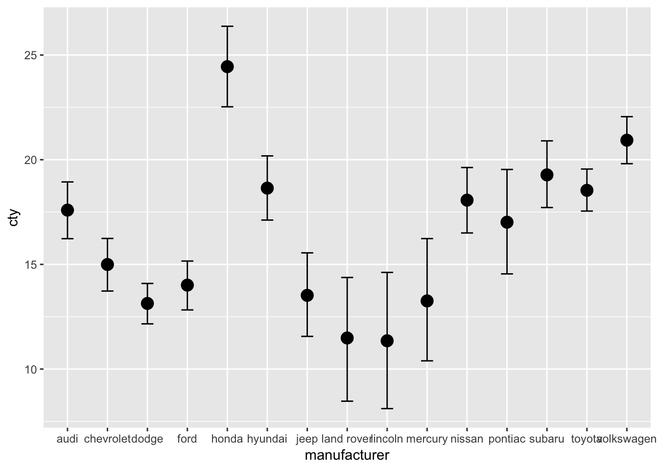

階層線形モデル

各群に回帰線を当てはめますが，その全体的な傾向も要約して表します。群ごとの散らばりを分布から作られているもの，と考えるところがミソです。

ランダム切片モデル

切片が群ごとに異なる，というモデルを考えます。今回は，15のメーカによって切片が違うとします。

result.hlm1 <- brm(cty~displ+(1|manufacturer),data=mpg)

## Compiling the C++ model

## Start sampling

## 
## SAMPLING FOR MODEL '9fac491b11fc784e76e04c51fb3d0c72' NOW (CHAIN 1).
## Chain 1: 
## Chain 1: Gradient evaluation took 4.6e-05 seconds
## Chain 1: 1000 transitions using 10 leapfrog steps per transition would take 0.46 seconds.
## Chain 1: Adjust your expectations accordingly!
## Chain 1: 
## Chain 1: 
## Chain 1: Iteration:    1 / 2000 [  0%]  (Warmup)
## Chain 1: Iteration:  200 / 2000 [ 10%]  (Warmup)
## Chain 1: Iteration:  400 / 2000 [ 20%]  (Warmup)
## Chain 1: Iteration:  600 / 2000 [ 30%]  (Warmup)
## Chain 1: Iteration:  800 / 2000 [ 40%]  (Warmup)
## Chain 1: Iteration: 1000 / 2000 [ 50%]  (Warmup)
## Chain 1: Iteration: 1001 / 2000 [ 50%]  (Sampling)
## Chain 1: Iteration: 1200 / 2000 [ 60%]  (Sampling)
## Chain 1: Iteration: 1400 / 2000 [ 70%]  (Sampling)
## Chain 1: Iteration: 1600 / 2000 [ 80%]  (Sampling)
## Chain 1: Iteration: 1800 / 2000 [ 90%]  (Sampling)
## Chain 1: Iteration: 2000 / 2000 [100%]  (Sampling)
## Chain 1: 
## Chain 1:  Elapsed Time: 0.316467 seconds (Warm-up)
## Chain 1:                0.27636 seconds (Sampling)
## Chain 1:                0.592827 seconds (Total)
## Chain 1: 
## 
## SAMPLING FOR MODEL '9fac491b11fc784e76e04c51fb3d0c72' NOW (CHAIN 2).
## Chain 2: 
## Chain 2: Gradient evaluation took 2.1e-05 seconds
## Chain 2: 1000 transitions using 10 leapfrog steps per transition would take 0.21 seconds.
## Chain 2: Adjust your expectations accordingly!
## Chain 2: 
## Chain 2: 
## Chain 2: Iteration:    1 / 2000 [  0%]  (Warmup)
## Chain 2: Iteration:  200 / 2000 [ 10%]  (Warmup)
## Chain 2: Iteration:  400 / 2000 [ 20%]  (Warmup)
## Chain 2: Iteration:  600 / 2000 [ 30%]  (Warmup)
## Chain 2: Iteration:  800 / 2000 [ 40%]  (Warmup)
## Chain 2: Iteration: 1000 / 2000 [ 50%]  (Warmup)
## Chain 2: Iteration: 1001 / 2000 [ 50%]  (Sampling)
## Chain 2: Iteration: 1200 / 2000 [ 60%]  (Sampling)
## Chain 2: Iteration: 1400 / 2000 [ 70%]  (Sampling)
## Chain 2: Iteration: 1600 / 2000 [ 80%]  (Sampling)
## Chain 2: Iteration: 1800 / 2000 [ 90%]  (Sampling)
## Chain 2: Iteration: 2000 / 2000 [100%]  (Sampling)
## Chain 2: 
## Chain 2:  Elapsed Time: 0.297376 seconds (Warm-up)
## Chain 2:                0.245653 seconds (Sampling)
## Chain 2:                0.543029 seconds (Total)
## Chain 2: 
## 
## SAMPLING FOR MODEL '9fac491b11fc784e76e04c51fb3d0c72' NOW (CHAIN 3).
## Chain 3: 
## Chain 3: Gradient evaluation took 1.9e-05 seconds
## Chain 3: 1000 transitions using 10 leapfrog steps per transition would take 0.19 seconds.
## Chain 3: Adjust your expectations accordingly!
## Chain 3: 
## Chain 3: 
## Chain 3: Iteration:    1 / 2000 [  0%]  (Warmup)
## Chain 3: Iteration:  200 / 2000 [ 10%]  (Warmup)
## Chain 3: Iteration:  400 / 2000 [ 20%]  (Warmup)
## Chain 3: Iteration:  600 / 2000 [ 30%]  (Warmup)
## Chain 3: Iteration:  800 / 2000 [ 40%]  (Warmup)
## Chain 3: Iteration: 1000 / 2000 [ 50%]  (Warmup)
## Chain 3: Iteration: 1001 / 2000 [ 50%]  (Sampling)
## Chain 3: Iteration: 1200 / 2000 [ 60%]  (Sampling)
## Chain 3: Iteration: 1400 / 2000 [ 70%]  (Sampling)
## Chain 3: Iteration: 1600 / 2000 [ 80%]  (Sampling)
## Chain 3: Iteration: 1800 / 2000 [ 90%]  (Sampling)
## Chain 3: Iteration: 2000 / 2000 [100%]  (Sampling)
## Chain 3: 
## Chain 3:  Elapsed Time: 0.30527 seconds (Warm-up)
## Chain 3:                0.246909 seconds (Sampling)
## Chain 3:                0.552179 seconds (Total)
## Chain 3: 
## 
## SAMPLING FOR MODEL '9fac491b11fc784e76e04c51fb3d0c72' NOW (CHAIN 4).
## Chain 4: 
## Chain 4: Gradient evaluation took 4e-05 seconds
## Chain 4: 1000 transitions using 10 leapfrog steps per transition would take 0.4 seconds.
## Chain 4: Adjust your expectations accordingly!
## Chain 4: 
## Chain 4: 
## Chain 4: Iteration:    1 / 2000 [  0%]  (Warmup)
## Chain 4: Iteration:  200 / 2000 [ 10%]  (Warmup)
## Chain 4: Iteration:  400 / 2000 [ 20%]  (Warmup)
## Chain 4: Iteration:  600 / 2000 [ 30%]  (Warmup)
## Chain 4: Iteration:  800 / 2000 [ 40%]  (Warmup)
## Chain 4: Iteration: 1000 / 2000 [ 50%]  (Warmup)
## Chain 4: Iteration: 1001 / 2000 [ 50%]  (Sampling)
## Chain 4: Iteration: 1200 / 2000 [ 60%]  (Sampling)
## Chain 4: Iteration: 1400 / 2000 [ 70%]  (Sampling)
## Chain 4: Iteration: 1600 / 2000 [ 80%]  (Sampling)
## Chain 4: Iteration: 1800 / 2000 [ 90%]  (Sampling)
## Chain 4: Iteration: 2000 / 2000 [100%]  (Sampling)
## Chain 4: 
## Chain 4:  Elapsed Time: 0.305949 seconds (Warm-up)
## Chain 4:                0.251213 seconds (Sampling)
## Chain 4:                0.557162 seconds (Total)
## Chain 4:

結果は次の通り。

# 結果（要約）
result.hlm1

##  Family: gaussian 
##   Links: mu = identity; sigma = identity 
## Formula: cty ~ displ + (1 | manufacturer) 
##    Data: mpg (Number of observations: 234) 
## Samples: 4 chains, each with iter = 2000; warmup = 1000; thin = 1;
##          total post-warmup samples = 4000
## 
## Group-Level Effects: 
## ~manufacturer (Number of levels: 15) 
##               Estimate Est.Error l-95% CI u-95% CI Eff.Sample Rhat
## sd(Intercept)     1.52      0.41     0.89     2.45       1225 1.00
## 
## Population-Level Effects: 
##           Estimate Est.Error l-95% CI u-95% CI Eff.Sample Rhat
## Intercept    25.51      0.77    23.98    26.96       2074 1.00
## displ        -2.49      0.18    -2.85    -2.15       3053 1.00
## 
## Family Specific Parameters: 
##       Estimate Est.Error l-95% CI u-95% CI Eff.Sample Rhat
## sigma     2.28      0.11     2.08     2.50       4543 1.00
## 
## Samples were drawn using sampling(NUTS). For each parameter, Eff.Sample 
## is a crude measure of effective sample size, and Rhat is the potential 
## scale reduction factor on split chains (at convergence, Rhat = 1).

# 推定値
result.hlm1$fit

## Inference for Stan model: 9fac491b11fc784e76e04c51fb3d0c72.
## 4 chains, each with iter=2000; warmup=1000; thin=1; 
## post-warmup draws per chain=1000, total post-warmup draws=4000.
## 
##                                         mean se_mean   sd    2.5%     25%
## b_Intercept                            25.51    0.02 0.77   23.98   25.02
## b_displ                                -2.49    0.00 0.18   -2.85   -2.61
## sd_manufacturer__Intercept              1.52    0.01 0.41    0.89    1.23
## sigma                                   2.28    0.00 0.11    2.08    2.21
## r_manufacturer[audi,Intercept]         -1.36    0.01 0.66   -2.67   -1.78
## r_manufacturer[chevrolet,Intercept]     1.86    0.01 0.66    0.63    1.43
## r_manufacturer[dodge,Intercept]        -1.36    0.01 0.54   -2.48   -1.70
## r_manufacturer[ford,Intercept]         -0.18    0.01 0.59   -1.39   -0.57
## r_manufacturer[honda,Intercept]         2.49    0.02 0.87    0.85    1.88
## r_manufacturer[hyundai,Intercept]      -0.68    0.01 0.69   -2.05   -1.14
## r_manufacturer[jeep,Intercept]         -0.46    0.02 0.79   -2.04   -0.97
## r_manufacturer[land.rover,Intercept]   -2.04    0.02 1.06   -4.22   -2.73
## r_manufacturer[lincoln,Intercept]      -0.39    0.02 1.02   -2.41   -1.07
## r_manufacturer[mercury,Intercept]      -0.79    0.02 0.96   -2.75   -1.41
## r_manufacturer[nissan,Intercept]        0.60    0.01 0.70   -0.77    0.13
## r_manufacturer[pontiac,Intercept]       0.90    0.01 0.89   -0.80    0.29
## r_manufacturer[subaru,Intercept]       -0.08    0.01 0.69   -1.45   -0.54
## r_manufacturer[toyota,Intercept]        0.36    0.01 0.56   -0.70   -0.02
## r_manufacturer[volkswagen,Intercept]    0.95    0.01 0.62   -0.24    0.53
## lp__                                 -552.75    0.13 4.18 -562.11 -555.23
##                                          50%     75%   97.5% n_eff Rhat
## b_Intercept                            25.52   26.02   26.96  2074    1
## b_displ                                -2.49   -2.37   -2.15  3053    1
## sd_manufacturer__Intercept              1.46    1.74    2.45  1225    1
## sigma                                   2.28    2.35    2.50  4543    1
## r_manufacturer[audi,Intercept]         -1.34   -0.93   -0.07  2182    1
## r_manufacturer[chevrolet,Intercept]     1.86    2.30    3.20  2257    1
## r_manufacturer[dodge,Intercept]        -1.35   -0.99   -0.32  1840    1
## r_manufacturer[ford,Intercept]         -0.17    0.22    0.96  2212    1
## r_manufacturer[honda,Intercept]         2.46    3.06    4.29  2661    1
## r_manufacturer[hyundai,Intercept]      -0.68   -0.22    0.67  2686    1
## r_manufacturer[jeep,Intercept]         -0.46    0.08    1.08  2582    1
## r_manufacturer[land.rover,Intercept]   -2.02   -1.31   -0.05  3190    1
## r_manufacturer[lincoln,Intercept]      -0.39    0.30    1.60  4073    1
## r_manufacturer[mercury,Intercept]      -0.77   -0.15    1.07  3878    1
## r_manufacturer[nissan,Intercept]        0.59    1.05    2.00  2490    1
## r_manufacturer[pontiac,Intercept]       0.88    1.46    2.73  3632    1
## r_manufacturer[subaru,Intercept]       -0.09    0.39    1.27  2433    1
## r_manufacturer[toyota,Intercept]        0.36    0.72    1.47  1832    1
## r_manufacturer[volkswagen,Intercept]    0.95    1.34    2.17  1891    1
## lp__                                 -552.35 -549.81 -545.65   989    1
## 
## Samples were drawn using NUTS(diag_e) at Tue Mar  5 18:20:00 2019.
## For each parameter, n_eff is a crude measure of effective sample size,
## and Rhat is the potential scale reduction factor on split chains (at 
## convergence, Rhat=1).

# 作図
mpg %>% 
  cbind(fitted(result.hlm1)) %>% 
  select(cty, displ, manufacturer, y_hat = Estimate) %>% 
  ggplot(aes(displ, y_hat, color = manufacturer)) +
  geom_smooth(method = "lm", se = FALSE) +
  geom_point(aes(y = cty)) + ylab("cty")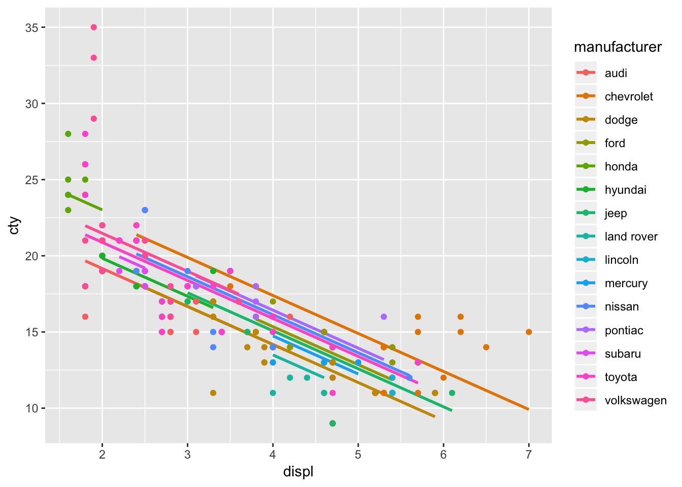

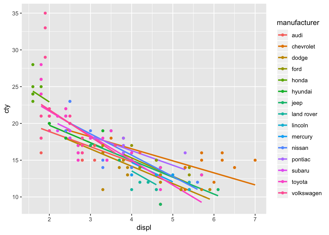
ランダム係数モデル

result.hlm2 <- brm(cty~displ+(displ|manufacturer),data=mpg)

## Compiling the C++ model

## Start sampling

## 
## SAMPLING FOR MODEL '53e4e9542f8ef009be512e8b26497a07' NOW (CHAIN 1).
## Chain 1: 
## Chain 1: Gradient evaluation took 6.7e-05 seconds
## Chain 1: 1000 transitions using 10 leapfrog steps per transition would take 0.67 seconds.
## Chain 1: Adjust your expectations accordingly!
## Chain 1: 
## Chain 1: 
## Chain 1: Iteration:    1 / 2000 [  0%]  (Warmup)
## Chain 1: Iteration:  200 / 2000 [ 10%]  (Warmup)
## Chain 1: Iteration:  400 / 2000 [ 20%]  (Warmup)
## Chain 1: Iteration:  600 / 2000 [ 30%]  (Warmup)
## Chain 1: Iteration:  800 / 2000 [ 40%]  (Warmup)
## Chain 1: Iteration: 1000 / 2000 [ 50%]  (Warmup)
## Chain 1: Iteration: 1001 / 2000 [ 50%]  (Sampling)
## Chain 1: Iteration: 1200 / 2000 [ 60%]  (Sampling)
## Chain 1: Iteration: 1400 / 2000 [ 70%]  (Sampling)
## Chain 1: Iteration: 1600 / 2000 [ 80%]  (Sampling)
## Chain 1: Iteration: 1800 / 2000 [ 90%]  (Sampling)
## Chain 1: Iteration: 2000 / 2000 [100%]  (Sampling)
## Chain 1: 
## Chain 1:  Elapsed Time: 1.30263 seconds (Warm-up)
## Chain 1:                1.36318 seconds (Sampling)
## Chain 1:                2.66581 seconds (Total)
## Chain 1: 
## 
## SAMPLING FOR MODEL '53e4e9542f8ef009be512e8b26497a07' NOW (CHAIN 2).
## Chain 2: 
## Chain 2: Gradient evaluation took 3.3e-05 seconds
## Chain 2: 1000 transitions using 10 leapfrog steps per transition would take 0.33 seconds.
## Chain 2: Adjust your expectations accordingly!
## Chain 2: 
## Chain 2: 
## Chain 2: Iteration:    1 / 2000 [  0%]  (Warmup)
## Chain 2: Iteration:  200 / 2000 [ 10%]  (Warmup)
## Chain 2: Iteration:  400 / 2000 [ 20%]  (Warmup)
## Chain 2: Iteration:  600 / 2000 [ 30%]  (Warmup)
## Chain 2: Iteration:  800 / 2000 [ 40%]  (Warmup)
## Chain 2: Iteration: 1000 / 2000 [ 50%]  (Warmup)
## Chain 2: Iteration: 1001 / 2000 [ 50%]  (Sampling)
## Chain 2: Iteration: 1200 / 2000 [ 60%]  (Sampling)
## Chain 2: Iteration: 1400 / 2000 [ 70%]  (Sampling)
## Chain 2: Iteration: 1600 / 2000 [ 80%]  (Sampling)
## Chain 2: Iteration: 1800 / 2000 [ 90%]  (Sampling)
## Chain 2: Iteration: 2000 / 2000 [100%]  (Sampling)
## Chain 2: 
## Chain 2:  Elapsed Time: 1.45759 seconds (Warm-up)
## Chain 2:                1.36186 seconds (Sampling)
## Chain 2:                2.81945 seconds (Total)
## Chain 2: 
## 
## SAMPLING FOR MODEL '53e4e9542f8ef009be512e8b26497a07' NOW (CHAIN 3).
## Chain 3: 
## Chain 3: Gradient evaluation took 5.9e-05 seconds
## Chain 3: 1000 transitions using 10 leapfrog steps per transition would take 0.59 seconds.
## Chain 3: Adjust your expectations accordingly!
## Chain 3: 
## Chain 3: 
## Chain 3: Iteration:    1 / 2000 [  0%]  (Warmup)
## Chain 3: Iteration:  200 / 2000 [ 10%]  (Warmup)
## Chain 3: Iteration:  400 / 2000 [ 20%]  (Warmup)
## Chain 3: Iteration:  600 / 2000 [ 30%]  (Warmup)
## Chain 3: Iteration:  800 / 2000 [ 40%]  (Warmup)
## Chain 3: Iteration: 1000 / 2000 [ 50%]  (Warmup)
## Chain 3: Iteration: 1001 / 2000 [ 50%]  (Sampling)
## Chain 3: Iteration: 1200 / 2000 [ 60%]  (Sampling)
## Chain 3: Iteration: 1400 / 2000 [ 70%]  (Sampling)
## Chain 3: Iteration: 1600 / 2000 [ 80%]  (Sampling)
## Chain 3: Iteration: 1800 / 2000 [ 90%]  (Sampling)
## Chain 3: Iteration: 2000 / 2000 [100%]  (Sampling)
## Chain 3: 
## Chain 3:  Elapsed Time: 1.555 seconds (Warm-up)
## Chain 3:                0.811949 seconds (Sampling)
## Chain 3:                2.36695 seconds (Total)
## Chain 3: 
## 
## SAMPLING FOR MODEL '53e4e9542f8ef009be512e8b26497a07' NOW (CHAIN 4).
## Chain 4: 
## Chain 4: Gradient evaluation took 2.9e-05 seconds
## Chain 4: 1000 transitions using 10 leapfrog steps per transition would take 0.29 seconds.
## Chain 4: Adjust your expectations accordingly!
## Chain 4: 
## Chain 4: 
## Chain 4: Iteration:    1 / 2000 [  0%]  (Warmup)
## Chain 4: Iteration:  200 / 2000 [ 10%]  (Warmup)
## Chain 4: Iteration:  400 / 2000 [ 20%]  (Warmup)
## Chain 4: Iteration:  600 / 2000 [ 30%]  (Warmup)
## Chain 4: Iteration:  800 / 2000 [ 40%]  (Warmup)
## Chain 4: Iteration: 1000 / 2000 [ 50%]  (Warmup)
## Chain 4: Iteration: 1001 / 2000 [ 50%]  (Sampling)
## Chain 4: Iteration: 1200 / 2000 [ 60%]  (Sampling)
## Chain 4: Iteration: 1400 / 2000 [ 70%]  (Sampling)
## Chain 4: Iteration: 1600 / 2000 [ 80%]  (Sampling)
## Chain 4: Iteration: 1800 / 2000 [ 90%]  (Sampling)
## Chain 4: Iteration: 2000 / 2000 [100%]  (Sampling)
## Chain 4: 
## Chain 4:  Elapsed Time: 1.36996 seconds (Warm-up)
## Chain 4:                1.19265 seconds (Sampling)
## Chain 4:                2.56261 seconds (Total)
## Chain 4:

## Warning: There were 13 divergent transitions after warmup. Increasing adapt_delta above 0.8 may help. See
## http://mc-stan.org/misc/warnings.html#divergent-transitions-after-warmup

## Warning: Examine the pairs() plot to diagnose sampling problems

結果は次の通り。

# 結果（要約）
result.hlm2

## Warning: There were 13 divergent transitions after warmup. Increasing adapt_delta above 0.8 may help.
## See http://mc-stan.org/misc/warnings.html#divergent-transitions-after-warmup

##  Family: gaussian 
##   Links: mu = identity; sigma = identity 
## Formula: cty ~ displ + (displ | manufacturer) 
##    Data: mpg (Number of observations: 234) 
## Samples: 4 chains, each with iter = 2000; warmup = 1000; thin = 1;
##          total post-warmup samples = 4000
## 
## Group-Level Effects: 
## ~manufacturer (Number of levels: 15) 
##                      Estimate Est.Error l-95% CI u-95% CI Eff.Sample Rhat
## sd(Intercept)            3.20      1.04     1.48     5.52       1193 1.00
## sd(displ)                0.87      0.33     0.28     1.56        841 1.00
## cor(Intercept,displ)    -0.88      0.20    -0.99    -0.32        697 1.00
## 
## Population-Level Effects: 
##           Estimate Est.Error l-95% CI u-95% CI Eff.Sample Rhat
## Intercept    25.74      1.18    23.39    28.07       1836 1.00
## displ        -2.66      0.32    -3.31    -2.03       1783 1.00
## 
## Family Specific Parameters: 
##       Estimate Est.Error l-95% CI u-95% CI Eff.Sample Rhat
## sigma     2.20      0.11     1.99     2.43       3721 1.00
## 
## Samples were drawn using sampling(NUTS). For each parameter, Eff.Sample 
## is a crude measure of effective sample size, and Rhat is the potential 
## scale reduction factor on split chains (at convergence, Rhat = 1).

# 推定値
result.hlm2$fit

## Inference for Stan model: 53e4e9542f8ef009be512e8b26497a07.
## 4 chains, each with iter=2000; warmup=1000; thin=1; 
## post-warmup draws per chain=1000, total post-warmup draws=4000.
## 
##                                         mean se_mean   sd    2.5%     25%
## b_Intercept                            25.74    0.03 1.18   23.39   24.96
## b_displ                                -2.66    0.01 0.32   -3.31   -2.87
## sd_manufacturer__Intercept              3.20    0.03 1.04    1.48    2.48
## sd_manufacturer__displ                  0.87    0.01 0.33    0.28    0.65
## cor_manufacturer__Intercept__displ     -0.88    0.01 0.20   -0.99   -0.97
## sigma                                   2.20    0.00 0.11    1.99    2.12
## r_manufacturer[audi,Intercept]         -2.73    0.04 1.77   -6.34   -3.87
## r_manufacturer[chevrolet,Intercept]    -2.65    0.05 2.03   -6.50   -4.02
## r_manufacturer[dodge,Intercept]        -2.15    0.04 1.84   -6.11   -3.30
## r_manufacturer[ford,Intercept]         -0.45    0.04 2.31   -5.16   -1.92
## r_manufacturer[honda,Intercept]         4.51    0.05 1.96    1.02    3.13
## r_manufacturer[hyundai,Intercept]      -1.24    0.04 1.97   -5.32   -2.45
## r_manufacturer[jeep,Intercept]         -1.57    0.04 2.32   -6.41   -2.99
## r_manufacturer[land.rover,Intercept]    0.36    0.08 3.47   -6.45   -1.79
## r_manufacturer[lincoln,Intercept]      -0.05    0.05 2.77   -5.84   -1.66
## r_manufacturer[mercury,Intercept]      -0.53    0.05 2.91   -6.62   -2.35
## r_manufacturer[nissan,Intercept]        1.55    0.04 2.01   -2.41    0.20
## r_manufacturer[pontiac,Intercept]      -1.48    0.07 3.04   -7.93   -3.32
## r_manufacturer[subaru,Intercept]        0.20    0.04 2.18   -4.34   -1.08
## r_manufacturer[toyota,Intercept]        2.64    0.04 1.59   -0.34    1.52
## r_manufacturer[volkswagen,Intercept]    3.44    0.05 1.86    0.24    2.12
## r_manufacturer[audi,displ]              0.60    0.01 0.59   -0.48    0.20
## r_manufacturer[chevrolet,displ]         1.02    0.01 0.47    0.09    0.71
## r_manufacturer[dodge,displ]             0.31    0.01 0.45   -0.54    0.00
## r_manufacturer[ford,displ]              0.17    0.01 0.55   -0.86   -0.20
## r_manufacturer[honda,displ]            -1.00    0.02 0.78   -2.64   -1.50
## r_manufacturer[hyundai,displ]           0.29    0.01 0.67   -0.97   -0.14
## r_manufacturer[jeep,displ]              0.36    0.01 0.56   -0.67   -0.02
## r_manufacturer[land.rover,displ]       -0.48    0.02 0.85   -2.28   -0.99
## r_manufacturer[lincoln,displ]           0.00    0.01 0.62   -1.24   -0.39
## r_manufacturer[mercury,displ]           0.03    0.01 0.72   -1.38   -0.41
## r_manufacturer[nissan,displ]           -0.24    0.01 0.57   -1.38   -0.62
## r_manufacturer[pontiac,displ]           0.67    0.02 0.79   -0.71    0.12
## r_manufacturer[subaru,displ]           -0.05    0.01 0.75   -1.58   -0.47
## r_manufacturer[toyota,displ]           -0.69    0.01 0.46   -1.64   -0.99
## r_manufacturer[volkswagen,displ]       -1.00    0.02 0.67   -2.48   -1.42
## lp__                                 -569.93    0.18 5.60 -581.80 -573.52
##                                          50%     75%   97.5% n_eff Rhat
## b_Intercept                            25.76   26.50   28.07  1836 1.00
## b_displ                                -2.66   -2.45   -2.03  1783 1.00
## sd_manufacturer__Intercept              3.09    3.80    5.52  1193 1.00
## sd_manufacturer__displ                  0.84    1.06    1.56   841 1.00
## cor_manufacturer__Intercept__displ     -0.94   -0.87   -0.32   697 1.00
## sigma                                   2.20    2.27    2.43  3721 1.00
## r_manufacturer[audi,Intercept]         -2.66   -1.53    0.63  2365 1.00
## r_manufacturer[chevrolet,Intercept]    -2.68   -1.35    1.53  1409 1.00
## r_manufacturer[dodge,Intercept]        -2.07   -0.94    1.38  2635 1.00
## r_manufacturer[ford,Intercept]         -0.40    1.04    3.99  3052 1.00
## r_manufacturer[honda,Intercept]         4.45    5.77    8.53  1777 1.00
## r_manufacturer[hyundai,Intercept]      -1.15   -0.01    2.55  2985 1.00
## r_manufacturer[jeep,Intercept]         -1.41   -0.05    2.61  3328 1.00
## r_manufacturer[land.rover,Intercept]    0.27    2.51    7.44  2106 1.00
## r_manufacturer[lincoln,Intercept]       0.00    1.62    5.44  3276 1.00
## r_manufacturer[mercury,Intercept]      -0.44    1.30    5.06  4136 1.00
## r_manufacturer[nissan,Intercept]        1.52    2.88    5.56  2856 1.00
## r_manufacturer[pontiac,Intercept]      -1.30    0.55    4.08  2121 1.00
## r_manufacturer[subaru,Intercept]        0.22    1.49    4.71  2823 1.00
## r_manufacturer[toyota,Intercept]        2.58    3.70    5.82  1966 1.00
## r_manufacturer[volkswagen,Intercept]    3.36    4.63    7.36  1590 1.00
## r_manufacturer[audi,displ]              0.57    0.98    1.85  2078 1.00
## r_manufacturer[chevrolet,displ]         1.03    1.32    1.94  1400 1.00
## r_manufacturer[dodge,displ]             0.29    0.59    1.28  2394 1.00
## r_manufacturer[ford,displ]              0.15    0.51    1.31  2590 1.00
## r_manufacturer[honda,displ]            -0.99   -0.47    0.46  1423 1.00
## r_manufacturer[hyundai,displ]           0.26    0.69    1.69  3093 1.00
## r_manufacturer[jeep,displ]              0.32    0.72    1.55  2990 1.00
## r_manufacturer[land.rover,displ]       -0.43    0.06    1.10  2397 1.00
## r_manufacturer[lincoln,displ]          -0.01    0.38    1.29  3282 1.00
## r_manufacturer[mercury,displ]           0.01    0.49    1.49  4145 1.00
## r_manufacturer[nissan,displ]           -0.23    0.13    0.86  3014 1.00
## r_manufacturer[pontiac,displ]           0.60    1.15    2.38  2073 1.00
## r_manufacturer[subaru,displ]           -0.06    0.39    1.54  2921 1.00
## r_manufacturer[toyota,displ]           -0.68   -0.37    0.13  2106 1.00
## r_manufacturer[volkswagen,displ]       -0.96   -0.53    0.15  1449 1.00
## lp__                                 -569.62 -566.00 -559.85   992 1.01
## 
## Samples were drawn using NUTS(diag_e) at Tue Mar  5 18:20:45 2019.
## For each parameter, n_eff is a crude measure of effective sample size,
## and Rhat is the potential scale reduction factor on split chains (at 
## convergence, Rhat=1).

# 作図
mpg %>% 
  cbind(fitted(result.hlm2)) %>% 
  select(cty, displ, manufacturer, y_hat = Estimate) %>% 
  ggplot(aes(displ, y_hat, color = manufacturer)) +
  geom_smooth(method = "lm", se = FALSE) +
  geom_point(aes(y = cty)) + ylab("cty")

brmsパッケージを使って

準備

パッケージの読み込み

データ

可視化してみましょう

最尤法による回帰

回帰線のベイズ推定

結果のプロット

事後分布とトレースプロット

MCMCサンプルをみてみる

回帰線のグラフ

事後予測分布

事後予測分布

分析に使ったstanコードも出力できる

一般線形モデル

階層線形モデル

ランダム切片モデル

ランダム係数モデル