データを入力します。
## パッケージの読み込み
library(rstan)
library(tidyverse)
## データの準備
X <- c(-27.020,3.570,8.191,9.808,9.603,9.945,10.056)
sc7 <- list(N=NROW(X),X=X)
ソースコード
## data{
##   int<lower=0> N;
##   real X[N];
## }
##
## parameters{
##   real mu;
##   real<lower=0> sig[N];
## }
##
## model{
##   for(n in 1:N){
##     //likelihood
##     X[n] ~ normal(mu,sig[n]);
##     //prior
##     sig[n] ~ inv_gamma(0.0001,0.0001);
##   }
##   // prior
##   mu ~ normal(0,1000);
## }
推定
fit <- sampling(model,sc7,iter=3000,warmup=1000,chains=4,thin=1)
## Warning: There were 1917 divergent transitions after warmup. Increasing adapt_delta above 0.8 may help. See
## http://mc-stan.org/misc/warnings.html#divergent-transitions-after-warmup
## Warning: Examine the pairs() plot to diagnose sampling problems
##  表示
fit
## Inference for Stan model: SevenScientist.
## 4 chains, each with iter=3000; warmup=1000; thin=1;
## post-warmup draws per chain=2000, total post-warmup draws=8000.
##
##          mean se_mean      sd  2.5%   25%   50%   75%  97.5% n_eff Rhat
## mu       9.88    0.01    0.12  9.60  9.81  9.86  9.95  10.06   128 1.04
## sig[1] 199.66   36.85 1979.60 16.77 28.48 46.86 92.32 854.54  2885 1.00
## sig[2]  51.23   14.52  788.07  2.85  5.52  9.37 14.24 144.60  2947 1.00
## sig[3]  63.59   53.92 1727.89  0.81  1.63  2.58  5.44  61.07  1027 1.00
## sig[4]   0.60    0.12    6.57  0.00  0.01  0.12  0.30   3.06  3119 1.00
## sig[5]   8.42    7.19   58.91  0.01  0.17  0.37  0.80  14.13    67 1.07
## sig[6]   0.56    0.14    5.37  0.00  0.04  0.13  0.34   2.28  1566 1.00
## sig[7]   2.45    1.27   16.51  0.00  0.11  0.29  0.62  10.07   170 1.02
## lp__    -3.55    0.58    3.10 -9.96 -5.55 -3.46 -1.36   1.83    29 1.14
##
## Samples were drawn using NUTS(diag_e) at Tue Mar  5 18:21:19 2019.
## For each parameter, n_eff is a crude measure of effective sample size,
## and Rhat is the potential scale reduction factor on split chains (at
## convergence, Rhat=1).
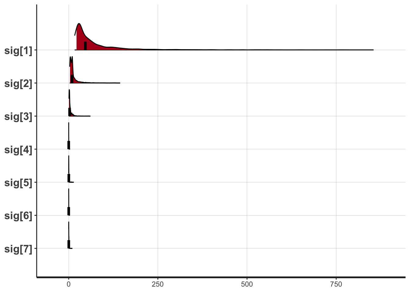
## 描画
plot(fit,pars=c("sig[1]","sig[2]","sig[3]","sig[4]",
                "sig[5]","sig[6]","sig[7]"),show_density=T)
## ci_level: 0.8 (80% intervals)
## outer_level: 0.95 (95% intervals)