Bayesian Network and Local Dependence Models
Source:vignettes/network-models.Rmd
network-models.RmdNote: Most examples in this vignette are shown with
eval=FALSEto keep CRAN build times short. For full rendered output, see the pkgdown site.
Bayesian Network Model (BNM)
BNM represents conditional probabilities between items in a network
format. A Directed Acyclic Graph (DAG) must be provided via
adj_matrix, adj_file, or g
(igraph object).
Creating the Graph
DAG <- matrix(
  c(
    "Item01", "Item02",
    "Item02", "Item03",
    "Item02", "Item04",
    "Item03", "Item05",
    "Item04", "Item05"
  ),
  ncol = 2, byrow = TRUE
)

# Graph object
g <- igraph::graph_from_data_frame(DAG)
g
#> IGRAPH 46a8093 DN-- 5 5 --
#> + attr: name (v/c)
#> + edges from 46a8093 (vertex names):
#> [1] Item01->Item02 Item02->Item03 Item02->Item04 Item03->Item05 Item04->Item05

# Adjacency matrix
adj_mat <- as.matrix(igraph::get.adjacency(g))
print(adj_mat)
#>        Item01 Item02 Item03 Item04 Item05
#> Item01      0      1      0      0      0
#> Item02      0      0      1      1      0
#> Item03      0      0      0      0      1
#> Item04      0      0      0      0      1
#> Item05      0      0      0      0      0
Running BNM
result.BNM <- BNM(J5S10, adj_matrix = adj_mat)
result.BNM
#> Adjacency Matrix
#>        Item01 Item02 Item03 Item04 Item05
#> Item01      0      1      0      0      0
#> Item02      0      0      1      1      0
#> Item03      0      0      0      0      1
#> Item04      0      0      0      0      1
#> Item05      0      0      0      0      0
#> [1] "Your graph is an acyclic graph."
#> [1] "Your graph is connected DAG."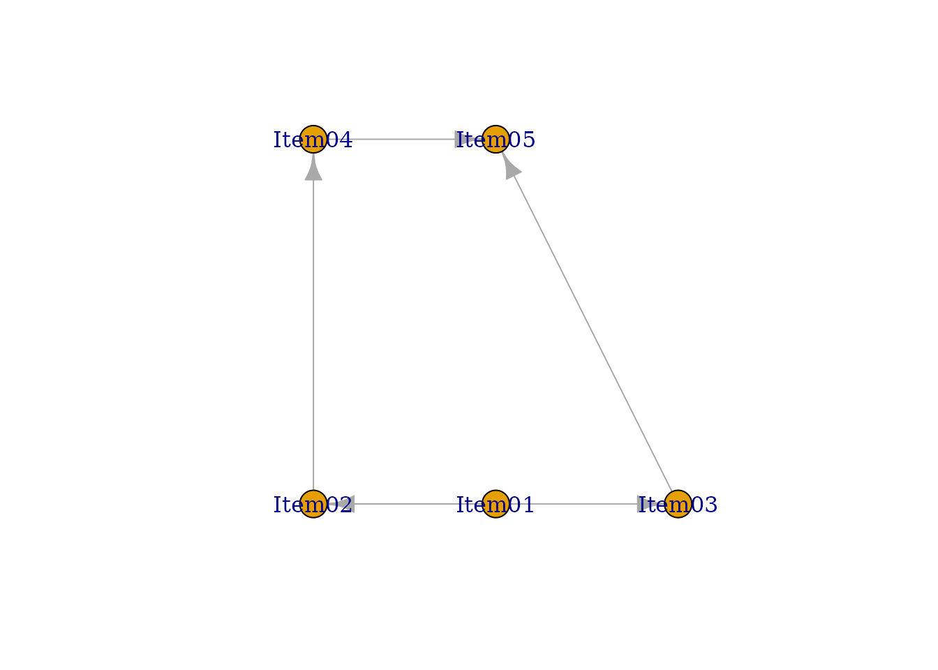
#>
#> Parameter Learning
#>        PIRP 1 PIRP 2 PIRP 3 PIRP 4
#> Item01  0.600
#> Item02  0.250    0.5
#> Item03  0.833    1.0
#> Item04  0.167    0.5
#> Item05  0.000    NaN  0.333  0.667
#>
#> Conditional Correct Response Rate
#>    Child Item N of Parents   Parent Items       PIRP Conditional CRR
#> 1      Item01            0     No Parents No Pattern           0.600
#> 2      Item02            1         Item01          0           0.250
#> 3      Item02            1         Item01          1           0.500
#> 4      Item03            1         Item02          0           0.833
#> 5      Item03            1         Item02          1           1.000
#> 6      Item04            1         Item02          0           0.167
#> 7      Item04            1         Item02          1           0.500
#> 8      Item05            2 Item03, Item04         00           0.000
#> 9      Item05            2 Item03, Item04         01              NA
#> 10     Item05            2 Item03, Item04         10           0.333
#> 11     Item05            2 Item03, Item04         11           0.667
#>
#> Model Fit Indices
#>                  value
#> model_log_like -27.046
#> bench_log_like  -8.935
#> null_log_like  -28.882
#> model_Chi_sq    36.222
#> null_Chi_sq     39.894
#> model_df        20.000
#> null_df         25.000
#> NFI              0.092
#> RFI              0.000
#> IFI              0.185
#> TLI              0.000
#> CFI              0.000
#> RMSEA            0.300
#> AIC             -3.778
#> CAIC           -29.829
#> BIC             -9.829
Structure Learning with Genetic Algorithm
BNM_GA() searches for a DAG suitable for the data using
a genetic algorithm:
BNM_GA(J5S10,
  population = 20, Rs = 0.5, Rm = 0.002, maxParents = 2,
  maxGeneration = 100, crossover = 2, elitism = 2
)
Structure Learning with PBIL
BNM_PBIL(J5S10,
  population = 20, Rs = 0.5, Rm = 0.005, maxParents = 2,
  alpha = 0.05, estimate = 4
)
Local Dependence Latent Rank Analysis (LDLRA)
LDLRA combines LRA and BNM to analyze how item dependency networks change across latent ranks. A graph must be specified for each rank.
Setting Up Rank-Specific Graphs
Graphs can be provided via CSV file, adjacency matrix list, or igraph object list:
DAG_dat <- matrix(c(
  "From", "To", "Rank",
  "Item01", "Item02", 1,
  "Item04", "Item05", 1,
  "Item01", "Item02", 2,
  "Item02", "Item03", 2,
  "Item04", "Item05", 2,
  "Item08", "Item09", 2,
  "Item08", "Item10", 2,
  "Item09", "Item10", 2,
  "Item08", "Item11", 2,
  "Item01", "Item02", 3,
  "Item02", "Item03", 3,
  "Item04", "Item05", 3,
  "Item08", "Item09", 3,
  "Item08", "Item10", 3,
  "Item09", "Item10", 3,
  "Item08", "Item11", 3,
  "Item02", "Item03", 4,
  "Item04", "Item06", 4,
  "Item04", "Item07", 4,
  "Item05", "Item06", 4,
  "Item05", "Item07", 4,
  "Item08", "Item10", 4,
  "Item08", "Item11", 4,
  "Item09", "Item11", 4,
  "Item02", "Item03", 5,
  "Item04", "Item06", 5,
  "Item04", "Item07", 5,
  "Item05", "Item06", 5,
  "Item05", "Item07", 5,
  "Item09", "Item11", 5,
  "Item10", "Item11", 5,
  "Item10", "Item12", 5
), ncol = 3, byrow = TRUE)

edgeFile <- tempfile(fileext = ".csv")
write.csv(DAG_dat, edgeFile, row.names = FALSE, quote = TRUE)
Running LDLRA
result.LDLRA <- LDLRA(J12S5000, ncls = 5, adj_file = edgeFile)
result.LDLRAStructure Learning for LDLRA with PBIL
LDLRA_PBIL() learns item-interaction graphs for each
rank automatically:
result.LDLRA.PBIL <- LDLRA_PBIL(J35S515,
  seed = 123, ncls = 5, method = "R",
  elitism = 1, successiveLimit = 15
)
result.LDLRA.PBIL
Local Dependence Biclustering (LDB)
LDB combines biclustering with Bayesian network models, analyzing relationships between item fields within each rank.
conf <- c(
  1, 6, 6, 8, 9, 9, 4, 7, 7, 7, 5, 8, 9, 10, 10,
  9, 9, 10, 10, 10, 2, 2, 3, 3, 5, 5, 6, 9, 9, 10,
  1, 1, 7, 9, 10
)

edges_data <- data.frame(
  "From Field (Parent) >>>" = c(
    6, 4, 5, 1, 1, 4,
    3, 4, 6, 2, 4, 4,
    3, 6, 4, 1,
    7, 9, 6, 7
  ),
  ">>> To Field (Child)" = c(
    8, 7, 8, 7, 2, 5,
    5, 8, 8, 4, 6, 7,
    5, 8, 5, 8,
    10, 10, 8, 9
  ),
  "At Class/Rank (Locus)" = c(
    2, 2, 2, 2, 2, 2,
    3, 3, 3, 3, 3, 3,
    4, 4, 4, 4,
    5, 5, 5, 5
  )
)

edgeFile <- tempfile(fileext = ".csv")
write.csv(edges_data, file = edgeFile, row.names = FALSE)
result.LDB <- LDB(U = J35S515, ncls = 5, conf = conf, adj_file = edgeFile)
result.LDB
plot(result.LDB, type = "Array")
plot(result.LDB, type = "TRP")
plot(result.LDB, type = "LRD")
plot(result.LDB, type = "RMP", students = 1:9, nc = 3, nr = 3)
plot(result.LDB, type = "FRP", nc = 3, nr = 2)
FieldPIRP visualizes correct answer counts for each rank and field:
plot(result.LDB, type = "FieldPIRP")Bicluster Network Model (BINET)
BINET combines biclustering with class-level network analysis. Unlike LDB where nodes are fields, in BINET the nodes represent classes.
conf <- c(
  1, 5, 5, 5, 9, 9, 6, 6, 6, 6, 2, 7, 7, 11, 11,
  7, 7, 12, 12, 12, 2, 2, 3, 3, 4, 4, 4, 8, 8, 12,
  1, 1, 6, 10, 10
)

edges_data <- data.frame(
  "From Class (Parent) >>>" = c(
    1, 2, 3, 4, 5, 7,
    2, 4, 6, 8, 10,
    6, 6, 11, 8, 9, 12
  ),
  ">>> To Class (Child)" = c(
    2, 4, 5, 5, 6, 11,
    3, 7, 9, 12, 12,
    10, 8, 12, 12, 11, 13
  ),
  "At Field (Locus)" = c(
    1, 2, 2, 3, 4, 4,
    5, 5, 5, 5, 5,
    7, 8, 8, 9, 9, 12
  )
)

edgeFile <- tempfile(fileext = ".csv")
write.csv(edges_data, file = edgeFile, row.names = FALSE)
result.BINET <- BINET(
  U = J35S515, ncls = 13, nfld = 12,
  conf = conf, adj_file = edgeFile
)
print(result.BINET)
plot(result.BINET, type = "Array")
plot(result.BINET, type = "TRP")
plot(result.BINET, type = "LRD")
plot(result.BINET, type = "RMP", students = 1:9, nc = 3, nr = 3)
plot(result.BINET, type = "FRP", nc = 3, nr = 2)
LDPSR shows Passing Student Rates for locally dependent classes:
plot(result.BINET, type = "LDPSR", nc = 3, nr = 2)