Skip to contents

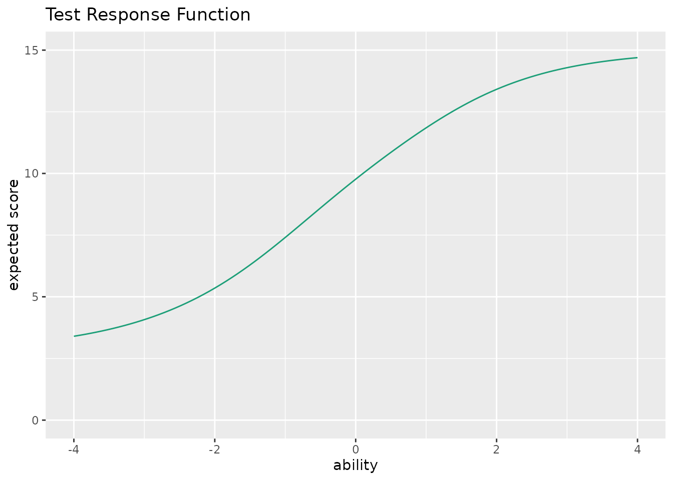
This function takes exametrika IRT output as input and generates a Test Response Function (TRF) using ggplot2. TRF shows the expected total score as a function of ability (theta).

Usage

plotTRF_gg(
  data,
  xvariable = c(-4, 4),
  title = TRUE,
  colors = NULL,
  linetype = "solid",
  show_legend = FALSE,
  legend_position = "right"
)

Arguments

data

An object of class c("exametrika", "IRT") from exametrika::IRT().

xvariable

A numeric vector of length 2 specifying the range of the x-axis (ability). Default is c(-4, 4).

title

Logical or character. If TRUE (default), display an auto-generated title. If FALSE, no title. If a character string, use it as a custom title.

colors

Character vector. Color(s) for the curve. If NULL (default), a colorblind-friendly palette is used.

linetype

Character or numeric specifying the line type. Default is "solid".

show_legend

Logical. If TRUE, display the legend. Default is FALSE.

legend_position

Character. Position of the legend. One of "right" (default), "top", "bottom", "left", "none".

Value

A single ggplot object showing the Test Response Function.

Details

The Test Response Function is the sum of all Item Characteristic Curves (ICCs). At each ability level, TRF represents the expected number of correct responses across all items. For a test with \(J\) items: $$TRF(\theta) = \sum_{j=1}^{J} P_j(\theta)$$

The y-axis ranges from 0 to the total number of items. The function supports 2PL, 3PL, and 4PL IRT models.

Examples

library(exametrika)
result <- IRT(J15S500, model = 3)
#> No ID column detected. All columns treated as response data. Sequential IDs (Student1, Student2, ...) were generated. Use id= parameter to specify the ID column explicitly.
#> 
iter 1 LogLik -3960.28                                                          
#> 
iter 2 LogLik -3938.35                                                          
#> 
iter 3 LogLik -3931.82                                                          
#> 
iter 4 LogLik -3928.68                                                          
#> 
iter 5 LogLik -3926.99                                                          
#> 
iter 6 LogLik -3926.05                                                          
#> 
iter 7 LogLik -3925.51                                                          
#> 
iter 8 LogLik -3925.19                                                          
#> 
iter 9 LogLik -3925.01                                                          
#> 
iter 10 LogLik -3924.9                                                          
#> 
iter 11 LogLik -3924.84                                                         
#> 
iter 12 LogLik -3924.8                                                          
#> 
iter 13 LogLik -3924.77                                                         
plot <- plotTRF_gg(result)
plot # Show Test Response Function