This function takes exametrika IRT output as input and generates Item Characteristic Curves (ICC) using ggplot2. ICC shows the probability of a correct response as a function of ability (theta).
Usage
plotICC_gg(
  data,
  items = NULL,
  xvariable = c(-4, 4),
  title = TRUE,
  colors = NULL,
  linetype = "solid",
  show_legend = FALSE,
  legend_position = "right"
)
Arguments
- data
An object of class
c("exametrika", "IRT")fromexametrika::IRT().- items
Numeric vector specifying which items to plot. If
NULL(default), all items are plotted.- xvariable
A numeric vector of length 2 specifying the range of the x-axis (ability). Default is
c(-4, 4).- title
Logical or character. If
TRUE(default), display an auto-generated title. IfFALSE, no title. If a character string, use it as a custom title (only for single-item plots).- colors
Character vector. Color(s) for the curve. If
NULL(default), a colorblind-friendly palette is used.- linetype
Character or numeric specifying the line type. Default is
"solid".- show_legend
Logical. If
TRUE, display the legend. Default isFALSE.- legend_position
Character. Position of the legend. One of
"right"(default),"top","bottom","left","none".
Value
A list of ggplot objects, one for each item. Each plot shows the Item Characteristic Curve for that item.
Details
The function supports 2PL, 3PL, and 4PL IRT models:
2PL: slope (a) and location (b) parameters
3PL: adds lower asymptote (c) parameter
4PL: adds upper asymptote (d) parameter
The ICC is computed using the four-parameter logistic model: $$P(\theta) = c + \frac{d - c}{1 + \exp(-a(\theta - b))}$$
Examples
library(exametrika)
result <- IRT(J15S500, model = 3)
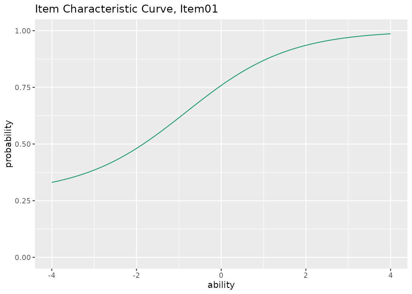
plots <- plotICC_gg(result)
plots[[1]] # Show ICC for the first item
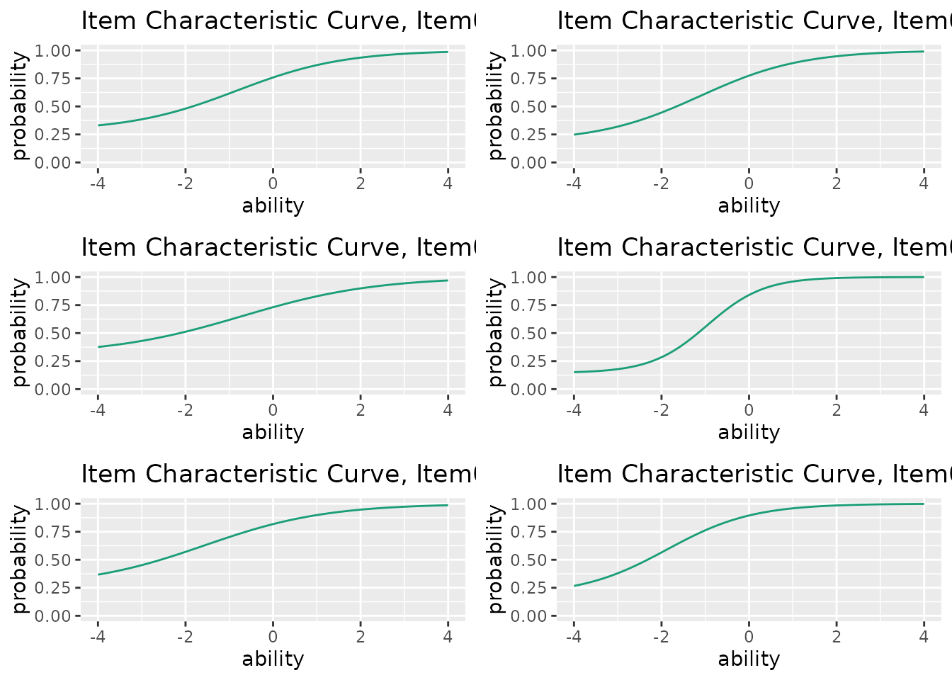
 combinePlots_gg(plots, selectPlots = 1:6) # Show first 6 items