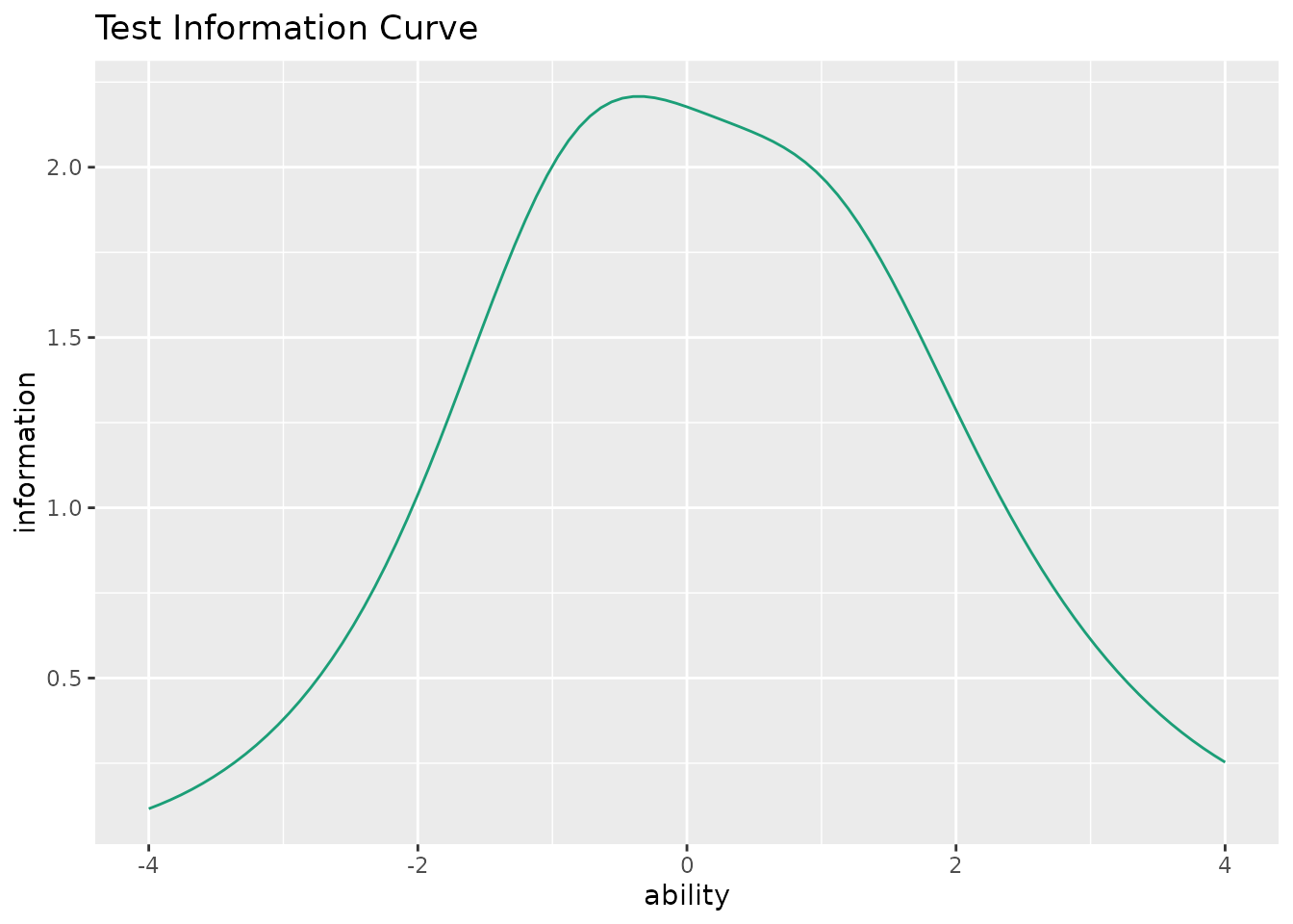
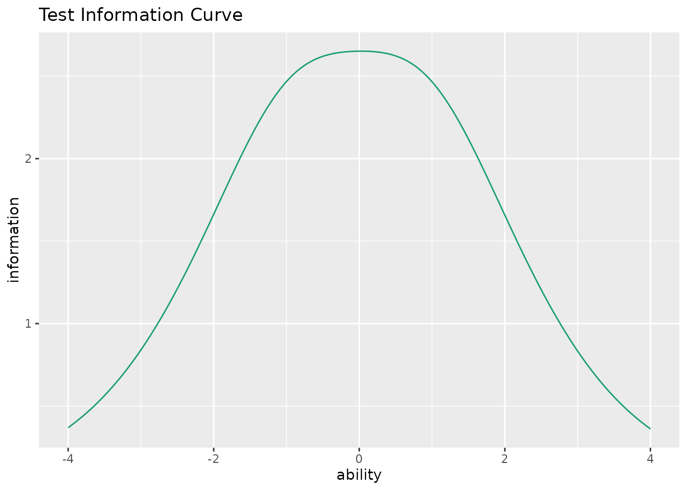
This function takes exametrika IRT or GRM output as input and generates a Test Information Curve (TIC) using ggplot2. TIC shows the total information provided by all items at each ability level.
Usage
plotTIC_gg(
  data,
  xvariable = c(-4, 4),
  title = TRUE,
  colors = NULL,
  linetype = "solid",
  show_legend = FALSE,
  legend_position = "right"
)
Arguments
- data
An object of class
c("exametrika", "IRT")fromexametrika::IRT()orc("exametrika", "GRM")fromexametrika::GRM().- xvariable
A numeric vector of length 2 specifying the range of the x-axis (ability). Default is
c(-4, 4).- title
Logical or character. If
TRUE(default), display an auto-generated title. IfFALSE, no title. If a character string, use it as a custom title.- colors
Character vector. Color(s) for the curve. If
NULL(default), a colorblind-friendly palette is used.- linetype
Character or numeric specifying the line type. Default is
"solid".- show_legend
Logical. If
TRUE, display the legend. Default isFALSE.- legend_position
Character. Position of the legend. One of
"right"(default),"top","bottom","left","none".
Details
The Test Information Function is the sum of all Item Information Functions. It indicates how precisely the test as a whole measures ability at each point on the theta scale. The reciprocal of test information is approximately equal to the squared standard error of measurement.
The function supports IRT models (2PL, 3PL, 4PL) and GRM.
Examples
library(exametrika)
# \donttest{
# IRT example
result_irt <- IRT(J15S500, model = 3)
plot_irt <- plotTIC_gg(result_irt)
plot_irt # Show Test Information Curve
 # GRM example
result_grm <- GRM(J5S1000)
plot_grm <- plotTIC_gg(result_grm)
plot_grm # Show Test Information Curve
# GRM example
result_grm <- GRM(J5S1000)
plot_grm <- plotTIC_gg(result_grm)
plot_grm # Show Test Information Curve
 # }
# }