Plot Rank Reference Vector (RRV) from exametrika

This function takes exametrika Biclustering output as input and generates a Rank Reference Vector (RRV) plot using ggplot2. RRV shows how each latent rank performs across fields, with one line per rank.

Supports both binary (2-valued) and polytomous (multi-valued) biclustering models. For polytomous data, the stat parameter controls how expected scores are calculated from category probabilities.

Usage

plotRRV_gg(
  data,
  title = TRUE,
  colors = NULL,
  linetype = "solid",
  show_legend = TRUE,
  legend_position = "right",
  stat = "mean",
  show_labels = NULL
)

Arguments

data

An object of class c("exametrika", "Biclustering") from exametrika::Biclustering().

title

Logical or character. If TRUE (default), display an auto-generated title. If FALSE, no title. If a character string, use it as a custom title.

colors

Character vector of colors for each rank. If NULL (default), a colorblind-friendly palette is used.

linetype

Character or numeric vector specifying the line types. If a single value, all lines use that type. If a vector, each rank uses the corresponding type. Default is "solid".

show_legend

Logical. If TRUE (default), display the legend.

legend_position

Character. Position of the legend. One of "right" (default), "top", "bottom", "left", "none".

stat

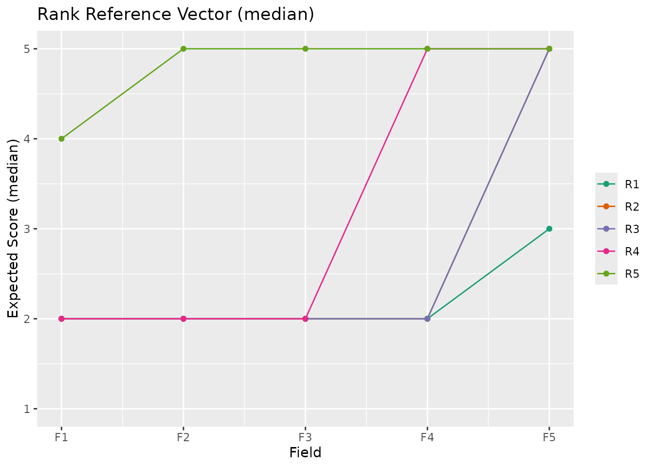
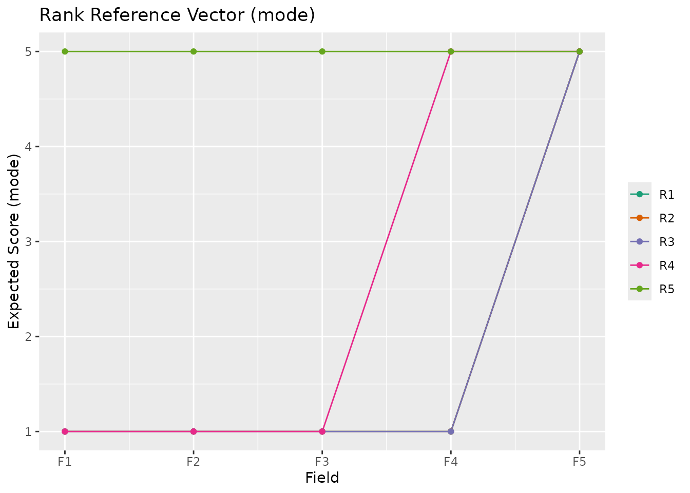
Character. Statistic for polytomous data: "mean" (default), "median", or "mode". For binary data, this parameter is ignored.

"mean": Expected score (sum of category x probability)
"median": Median category (cumulative probability >= 0.5)
"mode": Most probable category

show_labels

Logical. If TRUE, displays rank labels on each point using ggrepel to avoid overlaps. Defaults to FALSE since the legend already provides rank information.

Value

A single ggplot object showing the Rank Reference Vector.

Details

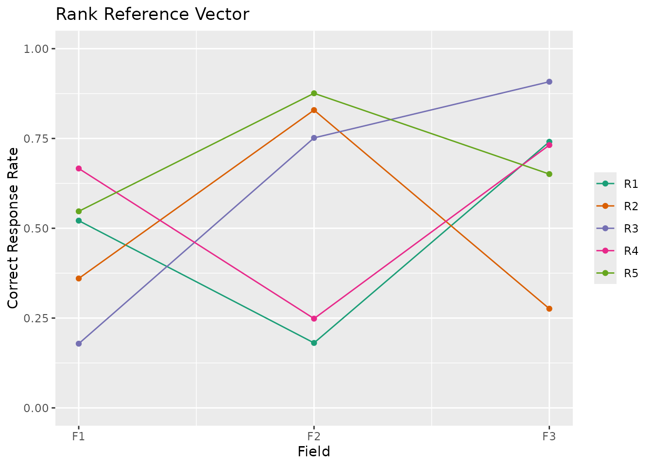
The Rank Reference Vector is the transpose of the Field Reference Profile (FRP). While FRP shows one plot per field, RRV displays all ranks in a single plot with fields on the x-axis. Each line represents a latent rank, showing its performance pattern across fields.

Binary Data (2 categories):

Y-axis shows "Correct Response Rate" (0.0 to 1.0)
Values represent the probability of correct response

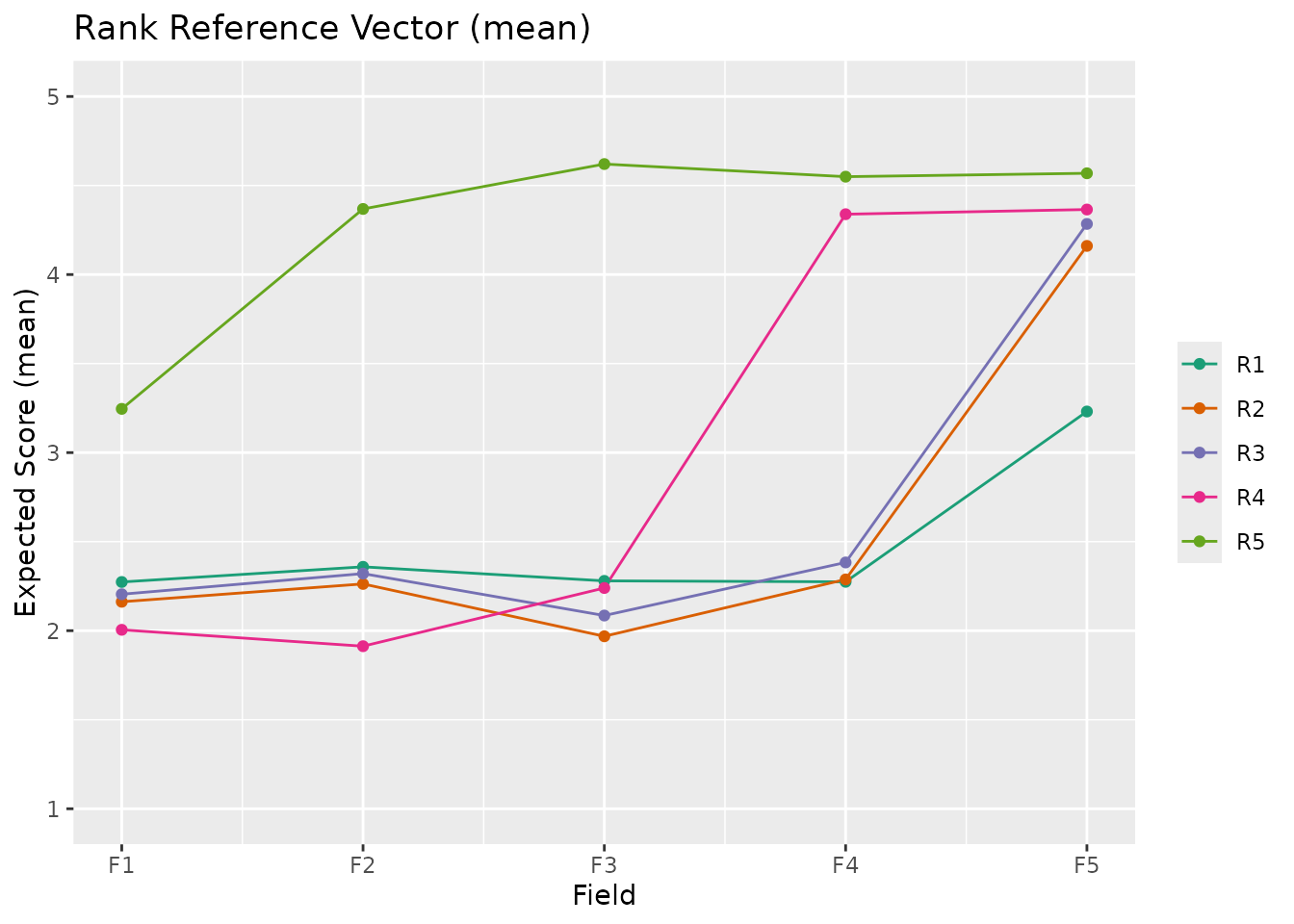
Polytomous Data (3+ categories):

Y-axis shows "Expected Score" (1 to max category)
Values are calculated using the stat parameter
Higher scores indicate better performance

RRV is used when latent ranks are ordinal (ordered). For unordered latent classes, use plotCRV_gg instead.

Examples

# Binary biclustering
library(exametrika)
result <- Biclustering(J15S500, nfld = 3, ncls = 5)
#> Biclustering is chosen.
#> 
iter 1 log_lik -4020.83                                                         
#> 
iter 2 log_lik -3997.76                                                         
#> 
iter 3 log_lik -3992.39                                                         
#> 
iter 4 log_lik -3986.8                                                          
#> 
iter 5 log_lik -3980                                                            
#> 
iter 6 log_lik -3973.35                                                         
#> 
iter 7 log_lik -3967.73                                                         
#> 
iter 8 log_lik -3963.4                                                          
#> 
iter 9 log_lik -3960.25                                                         
#> 
iter 10 log_lik -3958.04                                                        
#> 
iter 11 log_lik -3956.52                                                        
#> 
iter 12 log_lik -3955.47                                                        
#> 
iter 13 log_lik -3954.72                                                        
#> 
iter 14 log_lik -3954.17                                                        
#> 
iter 15 log_lik -3953.75                                                        
#> 
iter 16 log_lik -3953.39                                                        
#> 
#> 
#> Weakly ordinal alignment condition was satisfied.
#> No ID column detected. All columns treated as response data. Sequential IDs (Student1, Student2, ...) were generated. Use id= parameter to specify the ID column explicitly.
plotRRV_gg(result)


# \donttest{
# Ordinal biclustering (polytomous)
data(J35S500)
result_ord <- Biclustering(J35S500, ncls = 5, nfld = 5, method = "R")
#> Ranklustering is chosen.
#> 
iter 1 log_lik -22710.5                                                         
#> 
iter 2 log_lik -21311.9                                                         
#> 
iter 3 log_lik -21002.5                                                         
#> 
iter 4 log_lik -20945.8                                                         
#> 
iter 5 log_lik -20932.3                                                         
#> 
iter 6 log_lik -20929.2                                                         
#> 
iter 7 log_lik -20929.8                                                         
plotRRV_gg(result_ord) # Default: mean

plotRRV_gg(result_ord, stat = "median")

plotRRV_gg(result_ord, stat = "mode")


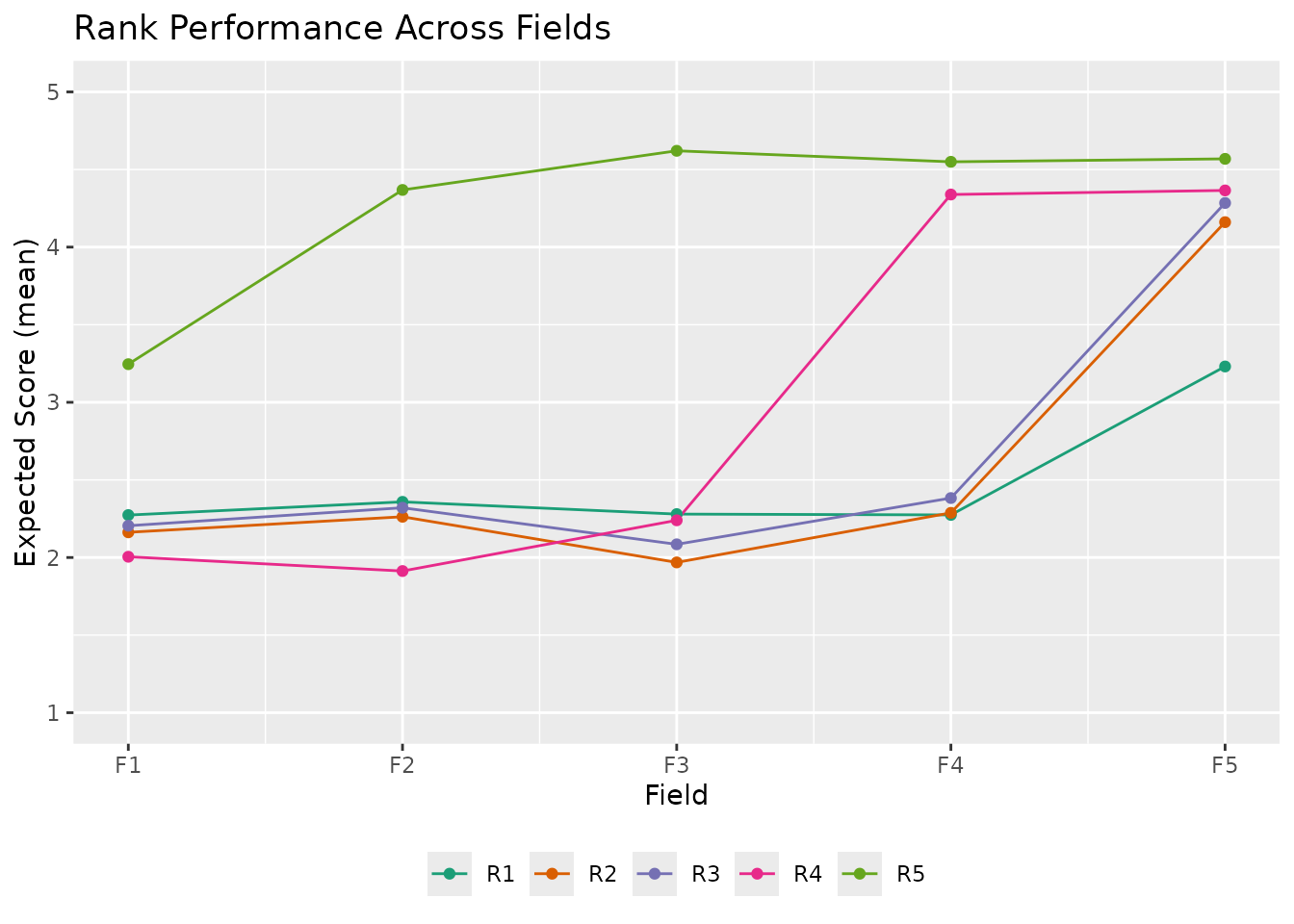
# Custom styling
plotRRV_gg(result_ord,
  title = "Rank Performance Across Fields",
  colors = c("#1b9e77", "#d95f02", "#7570b3", "#e7298a", "#66a61e"),
  legend_position = "bottom"
)

# }