U14. 多変量解析・行方向

ユニット概要

項目	内容
分類	枝（選択）
前提	U3（数学・行列の基礎）
次のユニット	U16（行と列をまたぐ分析）
使用データ	iris, psych::bfi
学習目標	PCAと因子分析の違いを理解する / Rで主成分分析・因子分析を実行し結果を解釈できる / SEMの基本概念（確認的因子分析）を理解し実行できる

---

事前知識

PCAと因子分析の違い

多変量データから少数の要約変数を得る手法として、主成分分析（PCA: Principal Component Analysis） と 因子分析（FA: Factor Analysis） があります。両者は似たような結果を返すことが多いですが、考え方が根本的に異なります。

主成分分析（PCA） は 次元削減 の手法です。観測変数の線形結合として主成分を構成し、データの分散を最大限保持しながら次元を減らします。主成分は観測変数から計算される合成変数であり、モデルの仮定はありません。

\[ z_1 = a_{11} x_1 + a_{12} x_2 + \cdots + a_{1p} x_p \]

因子分析（FA） は 潜在変数モデル です。直接観測できない潜在因子（共通因子）が観測変数の背後にあると仮定し、その因子を推定します。因子分析では観測変数は因子の結果（原因→結果の方向）であり、独自分散（uniqueness）の存在を認めます。

\[ x_j = \lambda_{j1} f_1 + \lambda_{j2} f_2 + \cdots + \lambda_{jm} f_m + u_j \]

	PCA	因子分析
目的	次元削減・要約	潜在構造の発見
方向	観測 → 主成分	因子 → 観測
分散	全分散を説明	共通分散のみ説明
独自性	なし	あり
Rの関数	prcomp()	psych::fa()

主成分分析（PCA）

prcomp()による実行

prcomp() は主成分分析を行うbase Rの関数です。引数 scale. = TRUE を指定すると、変数を標準化してから分析します（単位の異なる変数を扱う場合に推奨）。

# irisの数値列で主成分分析
pca_result <- prcomp(iris[, 1:4], scale. = TRUE)
summary(pca_result)

Importance of components:
                          PC1    PC2     PC3     PC4
Standard deviation     1.7084 0.9560 0.38309 0.14393
Proportion of Variance 0.7296 0.2285 0.03669 0.00518
Cumulative Proportion  0.7296 0.9581 0.99482 1.00000

出力の読み方:

• Standard deviation: 各主成分の標準偏差（固有値の平方根）
• Proportion of Variance: 各主成分が説明する分散の割合（寄与率）
• Cumulative Proportion: 累積寄与率（第2主成分まで約96%を説明）

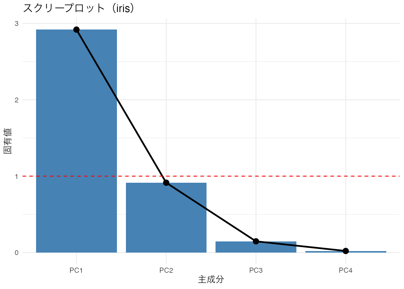
スクリープロット

固有値（各主成分の分散）を大きい順にプロットしたものを スクリープロット（scree plot） と呼びます。固有値が急激に減少する「肘（elbow）」の位置で主成分数を決定します。

# スクリープロット
eigenvalues <- pca_result$sdev^2
tibble(
  PC = paste0("PC", 1:length(eigenvalues)),
  Eigenvalue = eigenvalues
) %>%
  dplyr::mutate(PC = forcats::fct_inorder(PC)) %>%
  ggplot(aes(x = PC, y = Eigenvalue)) +
  geom_col(fill = "steelblue") +
  geom_line(aes(group = 1), linewidth = 1) +
  geom_point(size = 3) +
  geom_hline(yintercept = 1, linetype = "dashed", color = "red") +
  labs(title = "スクリープロット（iris）",
       x = "主成分", y = "固有値") +
  theme_minimal()

赤い破線は固有値 = 1 の基準線です（カイザー基準: 固有値が1以上の主成分を採用する目安）。

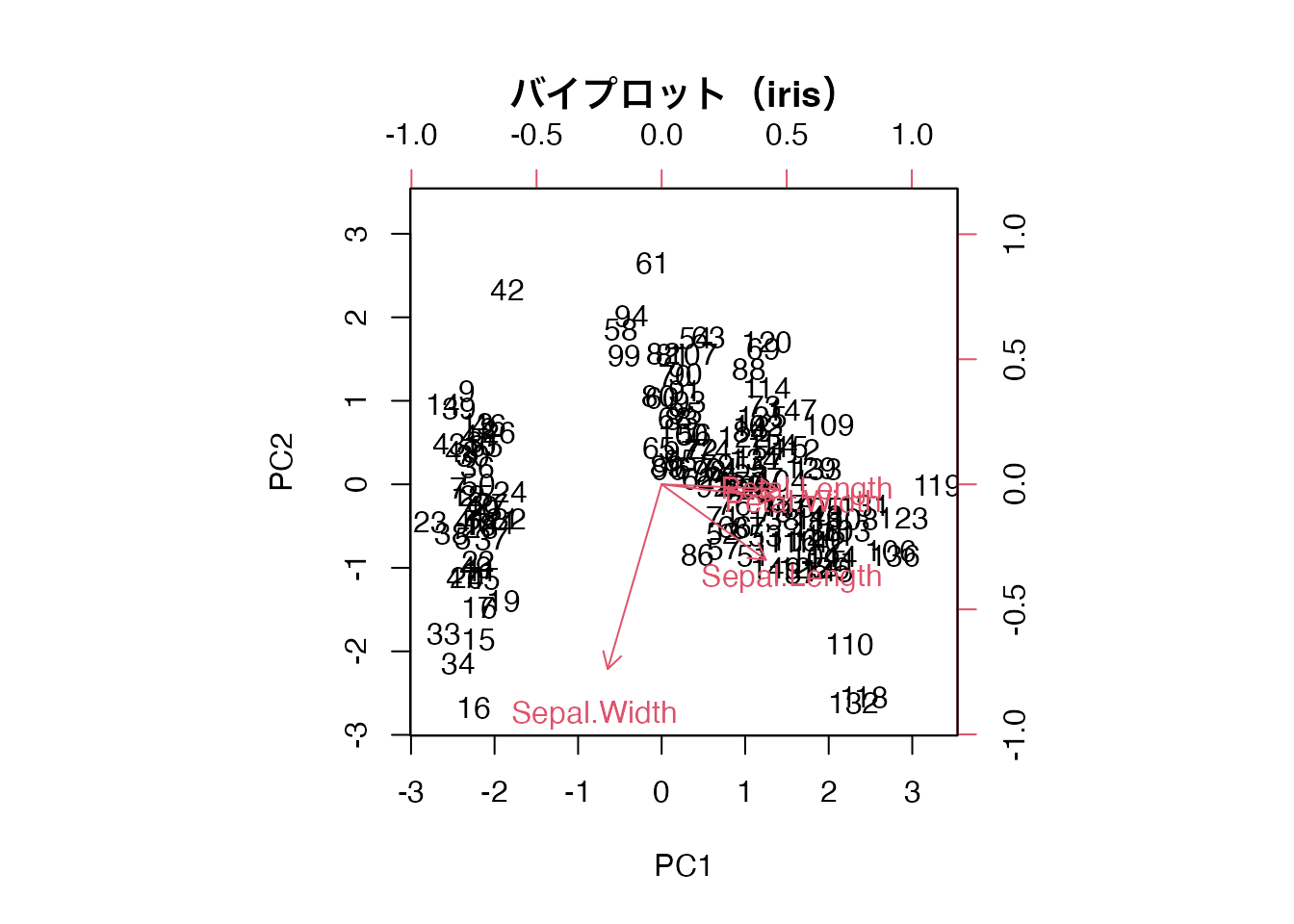
バイプロット

バイプロット（biplot） は、個体の主成分得点と変数の負荷量を同時にプロットした図です。

# バイプロット
biplot(pca_result, scale = 0,
       main = "バイプロット（iris）",
       xlab = "PC1", ylab = "PC2")

矢印が長い変数ほど主成分との関連が強く、矢印同士が近い方向を向く変数は互いに相関が高いことを示します。

因子分析

psych::fa()による実行

psych::fa() は因子分析を行う関数です。因子数 nfactors、回転法 rotate、推定法 fm を指定します。

pacman::p_load(psych)

# bfiデータの準備（欠損値を除去し、25項目を選択）
bfi_data <- psych::bfi[complete.cases(psych::bfi), 1:25]

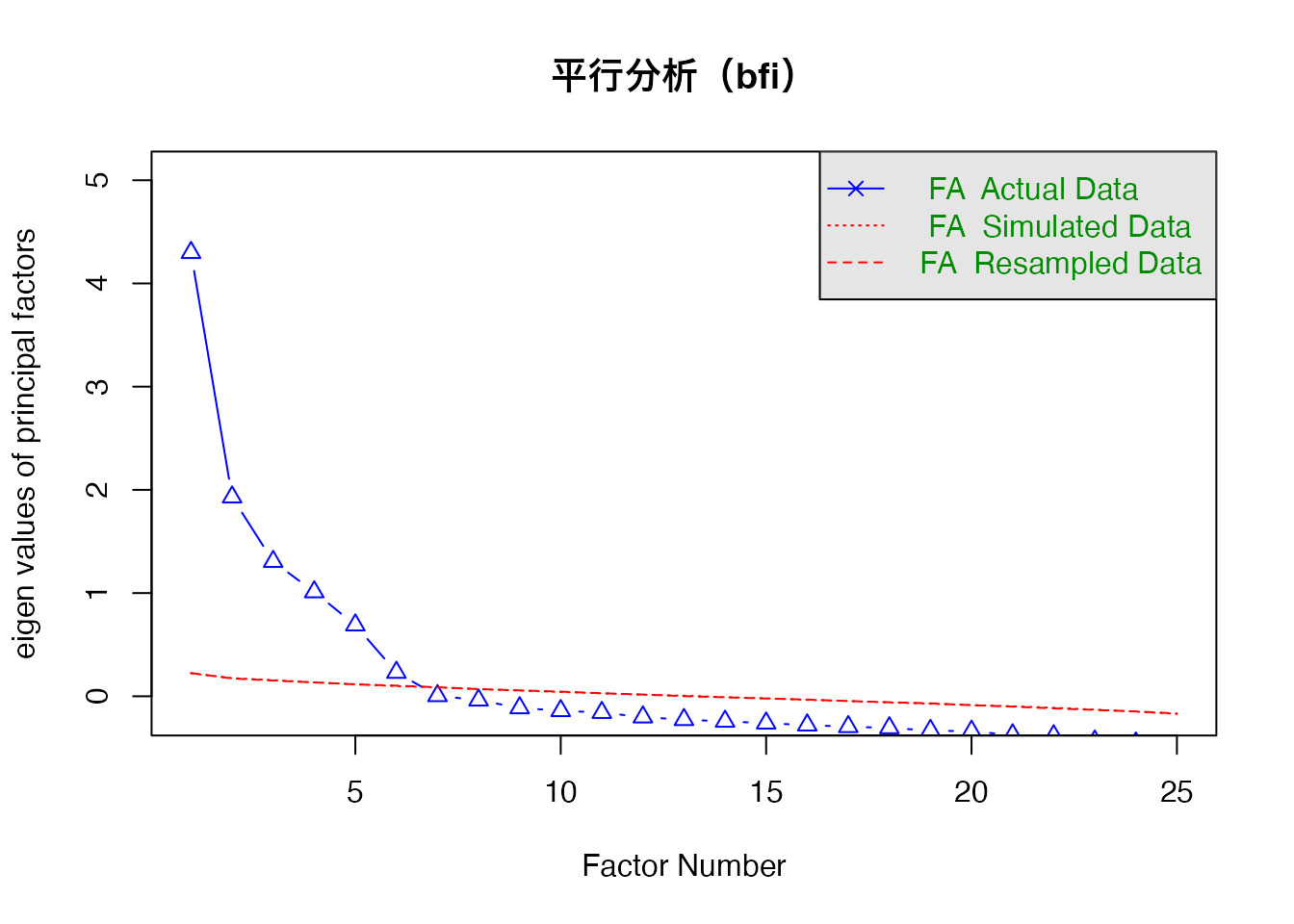
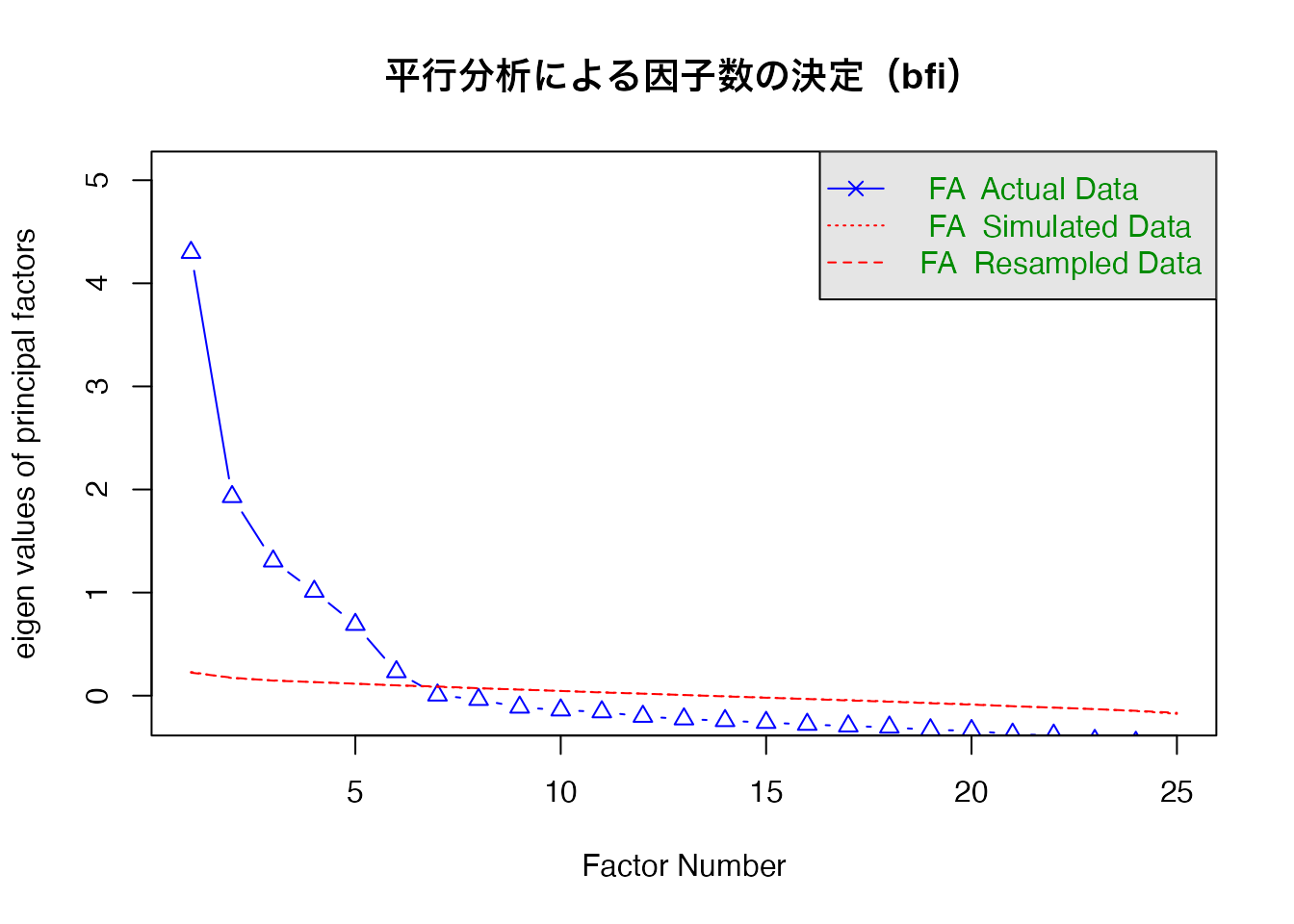
因子数の決定: 平行分析

因子数の決定には 平行分析（parallel analysis） が推奨されます。ランダムデータから得られる固有値と実データの固有値を比較し、実データの固有値がランダムデータを上回る因子数を採用します。

# 平行分析による因子数の決定
psych::fa.parallel(bfi_data, fa = "fa", main = "平行分析（bfi）")

Parallel analysis suggests that the number of factors =  6  and the number of components =  NA 

因子分析の実行

# 5因子・promax回転で因子分析
fa_result <- psych::fa(bfi_data, nfactors = 5, rotate = "promax", fm = "ml")
fa_result

Factor Analysis using method =  ml
Call: psych::fa(r = bfi_data, nfactors = 5, rotate = "promax", fm = "ml")
Standardized loadings (pattern matrix) based upon correlation matrix
     ML2   ML1   ML3   ML5   ML4   h2   u2 com
A1  0.14  0.11  0.05 -0.41 -0.05 0.16 0.84 1.5
A2  0.05  0.12  0.08  0.56 -0.02 0.40 0.60 1.2
A3  0.04  0.21  0.03  0.62 -0.01 0.52 0.48 1.3
A4 -0.02  0.09  0.19  0.43 -0.19 0.31 0.69 1.9
A5 -0.10  0.28 -0.03  0.54  0.01 0.48 0.52 1.6
C1  0.07 -0.05  0.55  0.00  0.17 0.33 0.67 1.2
C2  0.14 -0.13  0.66  0.09  0.06 0.42 0.58 1.2
C3  0.03 -0.09  0.59  0.08 -0.05 0.33 0.67 1.1
C4  0.14  0.03 -0.67  0.06 -0.03 0.48 0.52 1.1
C5  0.18 -0.09 -0.57  0.03  0.09 0.44 0.56 1.3
E1 -0.06 -0.64  0.16 -0.03 -0.04 0.36 0.64 1.2
E2  0.11 -0.71  0.05 -0.02 -0.02 0.55 0.45 1.1
E3  0.08  0.51 -0.06  0.22  0.26 0.46 0.54 2.0
E4 -0.03  0.61 -0.05  0.29 -0.10 0.54 0.46 1.5
E5  0.16  0.50  0.23  0.00  0.17 0.42 0.58 1.9
N1  0.88  0.23  0.03 -0.26 -0.10 0.72 0.28 1.4
N2  0.84  0.17  0.05 -0.25 -0.03 0.66 0.34 1.3
N3  0.72 -0.01  0.00 -0.01 -0.01 0.53 0.47 1.0
N4  0.49 -0.34 -0.10  0.07  0.09 0.50 0.50 2.0
N5  0.50 -0.16  0.01  0.15 -0.16 0.34 0.66 1.6
O1  0.00  0.16  0.04  0.01  0.51 0.32 0.68 1.2
O2  0.18  0.02 -0.08  0.15 -0.48 0.28 0.72 1.6
O3  0.04  0.27 -0.05  0.07  0.60 0.48 0.52 1.4
O4  0.15 -0.25 -0.03  0.16  0.37 0.24 0.76 2.6
O5  0.09  0.02 -0.03  0.04 -0.53 0.29 0.71 1.1

                       ML2  ML1  ML3  ML5  ML4
SS loadings           2.67 2.47 1.99 1.86 1.55
Proportion Var        0.11 0.10 0.08 0.07 0.06
Cumulative Var        0.11 0.21 0.28 0.36 0.42
Proportion Explained  0.25 0.23 0.19 0.18 0.15
Cumulative Proportion 0.25 0.49 0.68 0.85 1.00

 With factor correlations of 
      ML2   ML1   ML3  ML5  ML4
ML2  1.00 -0.28 -0.23 0.03 0.04
ML1 -0.28  1.00  0.40 0.33 0.12
ML3 -0.23  0.40  1.00 0.21 0.18
ML5  0.03  0.33  0.21 1.00 0.15
ML4  0.04  0.12  0.18 0.15 1.00

Mean item complexity =  1.4
Test of the hypothesis that 5 factors are sufficient.

df null model =  300  with the objective function =  7.41 with Chi Square =  16484.78
df of  the model are 185  and the objective function was  0.61 

The root mean square of the residuals (RMSR) is  0.03 
The df corrected root mean square of the residuals is  0.04 

The harmonic n.obs is  2236 with the empirical chi square  552.71  with prob <  2.7e-38 
The total n.obs was  2236  with Likelihood Chi Square =  1357.5  with prob <  1.9e-177 

Tucker Lewis Index of factoring reliability =  0.882
RMSEA index =  0.053  and the 90 % confidence intervals are  0.051 0.056
BIC =  -69.3
Fit based upon off diagonal values = 0.98
Measures of factor score adequacy             
                                                   ML2  ML1  ML3  ML5  ML4
Correlation of (regression) scores with factors   0.95 0.83 0.83 0.81 0.82
Multiple R square of scores with factors          0.91 0.70 0.70 0.66 0.67
Minimum correlation of possible factor scores     0.81 0.39 0.39 0.32 0.34

出力の読み方:

• Standardized loadings: 因子負荷量。各項目がどの因子にどの程度関連しているか
• h2: 共通性（communality）。因子によって説明される分散の割合
• u2: 独自性（uniqueness）。因子では説明されない分散の割合（\(u2 = 1 - h2\)）
• SS loadings: 各因子が説明する分散の合計
• Proportion Var: 各因子の寄与率

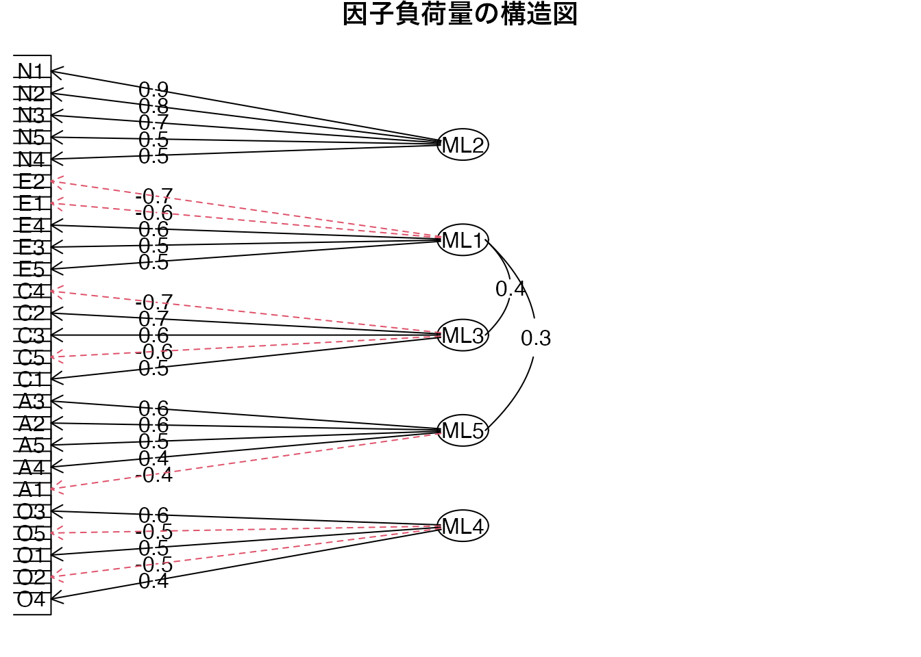
因子負荷量の可視化

# 因子負荷量の可視化
psych::fa.diagram(fa_result, main = "因子負荷量の構造図")

回転の種類

• varimax回転（直交回転）: 因子間の相関をゼロに保つ。解釈しやすいが現実にはやや制約が強い
• promax回転（斜交回転）: 因子間の相関を許容する。心理学では因子間に相関があることが多いため、promaxが好まれる

# varimax回転との比較
fa_varimax <- psych::fa(bfi_data, nfactors = 5, rotate = "varimax", fm = "ml")

# 因子間相関の比較
# promax: 因子間相関あり
fa_result$Phi

            ML2        ML1        ML3        ML5        ML4
ML2  1.00000000 -0.2810985 -0.2310369 0.02968499 0.04022075
ML1 -0.28109853  1.0000000  0.4016202 0.32843121 0.12463988
ML3 -0.23103688  0.4016202  1.0000000 0.21305038 0.17836221
ML5  0.02968499  0.3284312  0.2130504 1.00000000 0.15452583
ML4  0.04022075  0.1246399  0.1783622 0.15452583 1.00000000

promax回転では因子間相関行列 $Phi が得られます。varimax回転では因子間相関はゼロ（単位行列）です。

構造方程式モデリング（SEM）の概要

構造方程式モデリング（SEM: Structural Equation Modeling） は、潜在変数と観測変数の関係を柔軟にモデル化する枠組みです。因子分析の拡張として、確認的因子分析（CFA: Confirmatory Factor Analysis） がSEMの基本形です。

探索的因子分析（EFA）がデータ主導で因子構造を探索するのに対し、CFAは事前に仮定した因子構造が妥当かどうかを検証します。

lavaan::cfa()による実行

pacman::p_load(lavaan)

# CFAモデルの指定: Agreeableness因子にA1~A5が負荷
model <- 'A =~ A1 + A2 + A3 + A4 + A5'

# CFAの実行
cfa_result <- lavaan::cfa(model, data = bfi_data)
summary(cfa_result, fit.measures = TRUE, standardized = TRUE)

lavaan 0.6-21 ended normally after 32 iterations

  Estimator                                         ML
  Optimization method                           NLMINB
  Number of model parameters                        10

  Number of observations                          2236

Model Test User Model:
                                                      
  Test statistic                                73.043
  Degrees of freedom                                 5
  P-value (Chi-square)                           0.000

Model Test Baseline Model:

  Test statistic                              2101.436
  Degrees of freedom                                10
  P-value                                        0.000

User Model versus Baseline Model:

  Comparative Fit Index (CFI)                    0.967
  Tucker-Lewis Index (TLI)                       0.935

Loglikelihood and Information Criteria:

  Loglikelihood user model (H0)             -17817.725
  Loglikelihood unrestricted model (H1)     -17781.204
                                                      
  Akaike (AIC)                               35655.451
  Bayesian (BIC)                             35712.575
  Sample-size adjusted Bayesian (SABIC)      35680.804

Root Mean Square Error of Approximation:

  RMSEA                                          0.078
  90 Percent confidence interval - lower         0.063
  90 Percent confidence interval - upper         0.094
  P-value H_0: RMSEA <= 0.050                    0.002
  P-value H_0: RMSEA >= 0.080                    0.441

Standardized Root Mean Square Residual:

  SRMR                                           0.032

Parameter Estimates:

  Standard errors                             Standard
  Information                                 Expected
  Information saturated (h1) model          Structured

Latent Variables:
                   Estimate  Std.Err  z-value  P(>|z|)   Std.lv  Std.all
  A =~                                                                  
    A1                1.000                               0.517    0.371
    A2               -1.464    0.100  -14.622    0.000   -0.756   -0.654
    A3               -1.904    0.127  -14.986    0.000   -0.983   -0.763
    A4               -1.395    0.105  -13.335    0.000   -0.721   -0.498
    A5               -1.519    0.105  -14.445    0.000   -0.785   -0.625

Variances:
                   Estimate  Std.Err  z-value  P(>|z|)   Std.lv  Std.all
   .A1                1.670    0.053   31.778    0.000    1.670    0.862
   .A2                0.766    0.030   25.148    0.000    0.766    0.572
   .A3                0.695    0.038   18.396    0.000    0.695    0.418
   .A4                1.576    0.053   29.959    0.000    1.576    0.752
   .A5                0.961    0.036   26.420    0.000    0.961    0.609
    A                 0.267    0.034    7.946    0.000    1.000    1.000

出力の読み方:

• Latent Variables: 潜在変数から観測変数への因子負荷量（Estimate）
• Std.all: 標準化された因子負荷量（0.4以上が望ましい）
• 適合度指標: モデルがデータにどの程度適合しているか

主要な適合度指標

指標	良好な基準	意味
CFI（比較適合度指標）	0.95以上	独立モデルと比較したモデルの改善度
RMSEA（近似誤差二乗平均平方根）	0.06以下	モデルの近似の悪さの指標
SRMR（標準化残差二乗平均平方根）	0.08以下	観測相関と再現相関のずれ

これらの基準は目安であり、絶対的なものではありません。複数の指標を総合的に判断することが重要です。

---

ランクC: 基礎知識

14-C-1

主成分分析（PCA）は、観測変数の背後に潜在因子を仮定するモデルである。

TRUEFALSE

14-C-2

主成分分析で固有値が大きい主成分ほど、データの分散を多く説明している。

TRUEFALSE

14-C-3

因子分析における回転の目的は何か。

因子数を決定するため因子負荷量のパターンを解釈しやすくするため因子得点を計算するため共通性を最大化するため

14-C-4

因子負荷量が0.7のとき、その項目の共通性（\(h^2\)）はおよそいくらか（1因子の場合）。

0.300.490.701.00

14-C-5

CFI（比較適合度指標）が良好とされる一般的な基準はどれか。

0.80以上0.90以上0.95以上0.99以上

14-C-6

スクリープロットで主成分数を決める際、固有値のグラフのどこに注目するか。

固有値が最大の点固有値が急に減少する肘（elbow）の位置固有値がゼロになる点グラフの右端

14-C-7

因子分析における共通性（communality）とは何か。

因子間の相関係数共通因子によって説明される分散の割合すべての因子負荷量の合計独自因子の分散

14-C-8

RMSEAが低い値であるほど、モデルの適合が良いことを示す。

TRUEFALSE

---

ランクB: 実践スキル

14-B-1

iris データの数値4変数に対して prcomp(scale. = TRUE) で主成分分析を行い、summary() で結果を確認しなさい。第1主成分と第2主成分の累積寄与率を読み取ること。

pca_iris <- prcomp(iris[, 1:4], scale. = TRUE)
summary(pca_iris)

Importance of components:
                          PC1    PC2     PC3     PC4
Standard deviation     1.7084 0.9560 0.38309 0.14393
Proportion of Variance 0.7296 0.2285 0.03669 0.00518
Cumulative Proportion  0.7296 0.9581 0.99482 1.00000

• 第1主成分の寄与率: 約73%
• 第1・第2主成分の累積寄与率: 約96%
• 2つの主成分でデータの分散のほとんどを説明できることがわかります

第1主成分の負荷量（回転行列）を確認すると:

pca_iris$rotation

                    PC1         PC2        PC3        PC4
Sepal.Length  0.5210659 -0.37741762  0.7195664  0.2612863
Sepal.Width  -0.2693474 -0.92329566 -0.2443818 -0.1235096
Petal.Length  0.5804131 -0.02449161 -0.1421264 -0.8014492
Petal.Width   0.5648565 -0.06694199 -0.6342727  0.5235971

PC1は Petal.Length と Petal.Width に大きな正の負荷を持ち、花の「大きさ」を表す総合指標と解釈できます。

14-B-2

14-B-1の結果を使って、ggplot2でスクリープロットを作成しなさい。固有値 = 1 の基準線も描くこと。

eigenvalues <- pca_iris$sdev^2

tibble(
  PC = paste0("PC", seq_along(eigenvalues)),
  Eigenvalue = eigenvalues
) %>%
  dplyr::mutate(PC = forcats::fct_inorder(PC)) %>%
  ggplot(aes(x = PC, y = Eigenvalue)) +
  geom_col(fill = "steelblue", alpha = 0.7) +
  geom_line(aes(group = 1), linewidth = 1) +
  geom_point(size = 3) +
  geom_hline(yintercept = 1, linetype = "dashed", color = "red") +
  labs(title = "スクリープロット（iris）",
       x = "主成分", y = "固有値") +
  theme_minimal()

カイザー基準（固有値 > 1）では第1主成分のみが採用されますが、スクリープロットの肘の位置からは2主成分が妥当とも判断できます。

14-B-3

psych::bfi データ（欠損値除去後の25項目）に対して psych::fa.parallel() を実行し、推奨される因子数を確認しなさい。

bfi_data <- psych::bfi[complete.cases(psych::bfi), 1:25]

psych::fa.parallel(bfi_data, fa = "fa",
                   main = "平行分析による因子数の決定（bfi）")

Parallel analysis suggests that the number of factors =  6  and the number of components =  NA 

平行分析の結果、5因子または6因子が示唆されます。bfiデータはBig Five（外向性、協調性、誠実性、神経症傾向、開放性）の5因子を想定して設計されているため、5因子が理論的にも妥当です。

14-B-4

bfiデータに対して5因子のvarimax回転とpromax回転をそれぞれ実行し、因子負荷量のパターンを比較しなさい。

# varimax回転
fa_varimax <- psych::fa(bfi_data, nfactors = 5, rotate = "varimax", fm = "ml")

# promax回転
fa_promax <- psych::fa(bfi_data, nfactors = 5, rotate = "promax", fm = "ml")

# varimax回転の因子負荷量（上位の負荷量のみ表示）
psych::print.psych(fa_varimax, cut = 0.3, sort = TRUE)

Factor Analysis using method =  ml
Call: psych::fa(r = bfi_data, nfactors = 5, rotate = "varimax", fm = "ml")
Standardized loadings (pattern matrix) based upon correlation matrix
   item   ML2   ML1   ML3   ML5   ML4   h2   u2 com
N1   16  0.81                         0.72 0.28 1.2
N2   17  0.78                         0.66 0.34 1.1
N3   18  0.72                         0.53 0.47 1.0
N4   19  0.56 -0.37                   0.50 0.50 2.0
N5   20  0.52                         0.34 0.66 1.6
E2   12       -0.67                   0.55 0.45 1.4
E4   14        0.60        0.39       0.54 0.46 1.9
E1   11       -0.58                   0.36 0.64 1.2
E3   13        0.50        0.33  0.31 0.46 0.54 2.5
E5   15        0.50  0.31             0.42 0.58 2.3
C4    9             -0.65             0.48 0.52 1.3
C2    7              0.62             0.42 0.58 1.2
C5   10             -0.57             0.44 0.56 1.7
C3    8              0.56             0.33 0.67 1.1
C1    6              0.53             0.33 0.67 1.4
A3    3                    0.65       0.52 0.48 1.4
A5    5        0.34        0.58       0.48 0.52 1.8
A2    2                    0.58       0.40 0.60 1.4
A4    4                    0.45       0.31 0.69 2.0
A1    1                   -0.37       0.16 0.84 1.2
O3   23                          0.62 0.48 0.52 1.5
O5   25                         -0.52 0.29 0.71 1.1
O1   21                          0.52 0.32 0.68 1.4
O2   22                         -0.47 0.28 0.72 1.6
O4   24                          0.36 0.24 0.76 2.7

                       ML2  ML1  ML3  ML5  ML4
SS loadings           2.68 2.30 2.01 1.95 1.57
Proportion Var        0.11 0.09 0.08 0.08 0.06
Cumulative Var        0.11 0.20 0.28 0.36 0.42
Proportion Explained  0.26 0.22 0.19 0.19 0.15
Cumulative Proportion 0.26 0.47 0.67 0.85 1.00

Mean item complexity =  1.6
Test of the hypothesis that 5 factors are sufficient.

df null model =  300  with the objective function =  7.41 with Chi Square =  16484.78
df of  the model are 185  and the objective function was  0.61 

The root mean square of the residuals (RMSR) is  0.03 
The df corrected root mean square of the residuals is  0.04 

The harmonic n.obs is  2236 with the empirical chi square  552.71  with prob <  2.7e-38 
The total n.obs was  2236  with Likelihood Chi Square =  1357.5  with prob <  1.9e-177 

Tucker Lewis Index of factoring reliability =  0.882
RMSEA index =  0.053  and the 90 % confidence intervals are  0.051 0.056
BIC =  -69.3
Fit based upon off diagonal values = 0.98
Measures of factor score adequacy             
                                                   ML2  ML1  ML3  ML5  ML4
Correlation of (regression) scores with factors   0.93 0.87 0.86 0.85 0.83
Multiple R square of scores with factors          0.86 0.75 0.74 0.72 0.69
Minimum correlation of possible factor scores     0.73 0.51 0.48 0.43 0.39

# promax回転の因子負荷量
psych::print.psych(fa_promax, cut = 0.3, sort = TRUE)

Factor Analysis using method =  ml
Call: psych::fa(r = bfi_data, nfactors = 5, rotate = "promax", fm = "ml")
Standardized loadings (pattern matrix) based upon correlation matrix
   item   ML2   ML1   ML3   ML5   ML4   h2   u2 com
N1   16  0.88                         0.72 0.28 1.4
N2   17  0.84                         0.66 0.34 1.3
N3   18  0.72                         0.53 0.47 1.0
N5   20  0.50                         0.34 0.66 1.6
N4   19  0.49 -0.34                   0.50 0.50 2.0
E2   12       -0.71                   0.55 0.45 1.1
E1   11       -0.64                   0.36 0.64 1.2
E4   14        0.61                   0.54 0.46 1.5
E3   13        0.51                   0.46 0.54 2.0
E5   15        0.50                   0.42 0.58 1.9
C4    9             -0.67             0.48 0.52 1.1
C2    7              0.66             0.42 0.58 1.2
C3    8              0.59             0.33 0.67 1.1
C5   10             -0.57             0.44 0.56 1.3
C1    6              0.55             0.33 0.67 1.2
A3    3                    0.62       0.52 0.48 1.3
A2    2                    0.56       0.40 0.60 1.2
A5    5                    0.54       0.48 0.52 1.6
A4    4                    0.43       0.31 0.69 1.9
A1    1                   -0.41       0.16 0.84 1.5
O3   23                          0.60 0.48 0.52 1.4
O5   25                         -0.53 0.29 0.71 1.1
O1   21                          0.51 0.32 0.68 1.2
O2   22                         -0.48 0.28 0.72 1.6
O4   24                          0.37 0.24 0.76 2.6

                       ML2  ML1  ML3  ML5  ML4
SS loadings           2.67 2.47 1.99 1.86 1.55
Proportion Var        0.11 0.10 0.08 0.07 0.06
Cumulative Var        0.11 0.21 0.28 0.36 0.42
Proportion Explained  0.25 0.23 0.19 0.18 0.15
Cumulative Proportion 0.25 0.49 0.68 0.85 1.00

 With factor correlations of 
      ML2   ML1   ML3  ML5  ML4
ML2  1.00 -0.28 -0.23 0.03 0.04
ML1 -0.28  1.00  0.40 0.33 0.12
ML3 -0.23  0.40  1.00 0.21 0.18
ML5  0.03  0.33  0.21 1.00 0.15
ML4  0.04  0.12  0.18 0.15 1.00

Mean item complexity =  1.4
Test of the hypothesis that 5 factors are sufficient.

df null model =  300  with the objective function =  7.41 with Chi Square =  16484.78
df of  the model are 185  and the objective function was  0.61 

The root mean square of the residuals (RMSR) is  0.03 
The df corrected root mean square of the residuals is  0.04 

The harmonic n.obs is  2236 with the empirical chi square  552.71  with prob <  2.7e-38 
The total n.obs was  2236  with Likelihood Chi Square =  1357.5  with prob <  1.9e-177 

Tucker Lewis Index of factoring reliability =  0.882
RMSEA index =  0.053  and the 90 % confidence intervals are  0.051 0.056
BIC =  -69.3
Fit based upon off diagonal values = 0.98
Measures of factor score adequacy             
                                                   ML2  ML1  ML3  ML5  ML4
Correlation of (regression) scores with factors   0.95 0.83 0.83 0.81 0.82
Multiple R square of scores with factors          0.91 0.70 0.70 0.66 0.67
Minimum correlation of possible factor scores     0.81 0.39 0.39 0.32 0.34

# promax回転の因子間相関
fa_promax$Phi

            ML2        ML1        ML3        ML5        ML4
ML2  1.00000000 -0.2810985 -0.2310369 0.02968499 0.04022075
ML1 -0.28109853  1.0000000  0.4016202 0.32843121 0.12463988
ML3 -0.23103688  0.4016202  1.0000000 0.21305038 0.17836221
ML5  0.02968499  0.3284312  0.2130504 1.00000000 0.15452583
ML4  0.04022075  0.1246399  0.1783622 0.15452583 1.00000000

promax回転では因子間に相関が認められます。varimax回転は因子間の独立性を仮定するため、心理学データでは非現実的な場合があります。

14-B-5

promax回転の因子分析結果から、因子得点（factor scores）を抽出し、最初の6行を表示しなさい。

fa_promax <- psych::fa(bfi_data, nfactors = 5, rotate = "promax",
                       fm = "ml", scores = "regression")

# 因子得点の抽出
factor_scores <- fa_promax$scores

# 最初の6行を表示
head(factor_scores)

              ML2         ML1        ML3         ML5        ML4
61623  0.08862003  1.21884758  1.4035023  0.23747261  0.4542889
61629  0.56229860 -1.68813980 -1.2059063 -2.24941004 -0.6991252
61634 -0.15784382  0.25785108 -0.1693194 -0.08601393 -0.3591560
61640 -0.56483391 -0.01613539  0.5229984 -1.66407270 -0.2351623
61661 -0.83221381  0.22651913 -1.3085976  0.53781613  0.2517961
61664  1.11474343  0.22973095 -0.2390623  1.05440620  0.8927368

因子得点は各個体の各因子上での位置を表します。これを後続の分析（クラスタ分析、回帰分析の説明変数など）に利用できます。

14-B-6

lavaan パッケージを使って、bfiデータの Agreeableness 項目（A1〜A5）に対する確認的因子分析を実行し、適合度指標を確認しなさい。

pacman::p_load(lavaan)

# CFAモデルの指定
model <- 'A =~ A1 + A2 + A3 + A4 + A5'

# CFAの実行
cfa_result <- lavaan::cfa(model, data = bfi_data)

# 結果の要約（適合度指標と標準化推定値を含む）
summary(cfa_result, fit.measures = TRUE, standardized = TRUE)

lavaan 0.6-21 ended normally after 32 iterations

  Estimator                                         ML
  Optimization method                           NLMINB
  Number of model parameters                        10

  Number of observations                          2236

Model Test User Model:
                                                      
  Test statistic                                73.043
  Degrees of freedom                                 5
  P-value (Chi-square)                           0.000

Model Test Baseline Model:

  Test statistic                              2101.436
  Degrees of freedom                                10
  P-value                                        0.000

User Model versus Baseline Model:

  Comparative Fit Index (CFI)                    0.967
  Tucker-Lewis Index (TLI)                       0.935

Loglikelihood and Information Criteria:

  Loglikelihood user model (H0)             -17817.725
  Loglikelihood unrestricted model (H1)     -17781.204
                                                      
  Akaike (AIC)                               35655.451
  Bayesian (BIC)                             35712.575
  Sample-size adjusted Bayesian (SABIC)      35680.804

Root Mean Square Error of Approximation:

  RMSEA                                          0.078
  90 Percent confidence interval - lower         0.063
  90 Percent confidence interval - upper         0.094
  P-value H_0: RMSEA <= 0.050                    0.002
  P-value H_0: RMSEA >= 0.080                    0.441

Standardized Root Mean Square Residual:

  SRMR                                           0.032

Parameter Estimates:

  Standard errors                             Standard
  Information                                 Expected
  Information saturated (h1) model          Structured

Latent Variables:
                   Estimate  Std.Err  z-value  P(>|z|)   Std.lv  Std.all
  A =~                                                                  
    A1                1.000                               0.517    0.371
    A2               -1.464    0.100  -14.622    0.000   -0.756   -0.654
    A3               -1.904    0.127  -14.986    0.000   -0.983   -0.763
    A4               -1.395    0.105  -13.335    0.000   -0.721   -0.498
    A5               -1.519    0.105  -14.445    0.000   -0.785   -0.625

Variances:
                   Estimate  Std.Err  z-value  P(>|z|)   Std.lv  Std.all
   .A1                1.670    0.053   31.778    0.000    1.670    0.862
   .A2                0.766    0.030   25.148    0.000    0.766    0.572
   .A3                0.695    0.038   18.396    0.000    0.695    0.418
   .A4                1.576    0.053   29.959    0.000    1.576    0.752
   .A5                0.961    0.036   26.420    0.000    0.961    0.609
    A                 0.267    0.034    7.946    0.000    1.000    1.000

適合度指標の解釈:

• CFI: 0.95以上なら良好
• RMSEA: 0.06以下なら良好、信頼区間も確認
• SRMR: 0.08以下なら良好

5項目1因子モデルの適合度を総合的に判断してください。

14-B-7

14-B-6のCFAの結果をパス図で可視化しなさい。semPlot::semPaths() を使うこと（未インストールの場合は install.packages("semPlot") で導入）。

pacman::p_load(semPlot)

# パス図の描画
semPlot::semPaths(cfa_result,
                  what = "std",          # 標準化推定値を表示
                  layout = "tree",       # ツリー型レイアウト
                  edge.label.cex = 1.2,  # パス係数のフォントサイズ
                  sizeMan = 8,           # 観測変数ノードのサイズ
                  sizeLat = 10,          # 潜在変数ノードのサイズ
                  style = "lisrel",      # LISRELスタイル
                  nCharNodes = 3,        # ノードラベルの文字数
                  title = TRUE)
title("CFA: Agreeableness 1因子モデル")

パス図では、楕円が潜在変数（因子）、四角が観測変数、矢印の上の数値が標準化された因子負荷量を表します。semPlot パッケージがインストールされていない場合は、上記コードを実行する前に install.packages("semPlot") を実行してください。

14-B-8

irisの数値4変数に対してPCAと因子分析（1因子）の結果を比較しなさい。PCAの第1主成分の負荷量と、因子分析の因子負荷量の値を並べて確認すること。

# PCA
pca_iris <- prcomp(iris[, 1:4], scale. = TRUE)

# 因子分析（1因子）
fa_iris <- psych::fa(iris[, 1:4], nfactors = 1, rotate = "none", fm = "ml")

# 比較表の作成
comparison <- tibble(
  Variable = colnames(iris[, 1:4]),
  PCA_PC1 = pca_iris$rotation[, 1],
  FA_F1 = as.numeric(fa_iris$loadings[, 1])
)
comparison

# A tibble: 4 × 3
  Variable     PCA_PC1  FA_F1
  <chr>          <dbl>  <dbl>
1 Sepal.Length   0.521  0.872
2 Sepal.Width   -0.269 -0.422
3 Petal.Length   0.580  0.998
4 Petal.Width    0.565  0.965

PCAの負荷量と因子分析の因子負荷量は似た傾向を示しますが、値は異なります。PCAは全分散を対象にし、因子分析は共通分散のみを対象にするためです。特に共通性（communality）の低い変数では差が大きくなります。

# 共通性の確認
tibble(
  Variable = colnames(iris[, 1:4]),
  Communality = as.numeric(fa_iris$communalities),
  Uniqueness = as.numeric(fa_iris$uniquenesses)
)

# A tibble: 4 × 3
  Variable     Communality Uniqueness
  <chr>              <dbl>      <dbl>
1 Sepal.Length       0.760    0.240  
2 Sepal.Width        0.178    0.822  
3 Petal.Length       0.995    0.00490
4 Petal.Width        0.931    0.0693 

---

ランクA: AI協働

14-A-1

psych::bfi データ（または自分が興味のあるデータ）を使い、生成AIと協力して以下の因子分析の全工程を設計・実行してください。

1. AIに「このデータに適切な因子数は何か」を相談し、平行分析の結果と合わせて判断する
2. 因子分析を実行し、AIに因子負荷量の解釈を手伝ってもらう（どの項目がどの因子に負荷しているか、因子に名前を付ける）
3. 回転法の選択理由をAIに説明してもらう
4. 因子得点を算出し、因子間の散布図を描く
5. AIの解釈に対して、自分の知識と照らし合わせて批判的に検討する

AIの提案を 必ず自分で実行して確認 すること。AIが提案した因子名が心理学的に妥当か、自分でも考えてみましょう。

14-A-2

bfiデータの5因子モデルについて、生成AIと協力して測定モデルの評価を行ってください。

1. lavaanで5因子CFAモデルを指定する（A1-A5, C1-C5, E1-E5, N1-N5, O1-O5の各5項目が対応する因子に負荷）
2. モデルを推定し、適合度指標を確認する
3. 適合度が不十分な場合、AIに「どう改善すべきか」を相談する（例: 修正指標の活用、項目の削除、相関誤差の追加）
4. 改善前後のモデルを比較し、結果を報告する

注意: AIの提案をすべて受け入れるのではなく、理論的に正当化できるかどうかを自分で判断してください。

---

まとめ

このユニットで学んだこと:

• PCAと因子分析の違い: PCAは次元削減（データ要約）、因子分析は潜在変数モデル（構造の発見）。目的に応じて使い分ける
• 主成分分析: prcomp() で実行。スクリープロットで主成分数を判断し、バイプロットで解釈する
• 因子分析: psych::fa() で実行。平行分析で因子数を決定し、回転後の因子負荷量で構造を解釈する
• 回転法: varimax（直交）は因子間独立を仮定、promax（斜交）は因子間相関を許容。心理学データではpromaxが一般的
• 確認的因子分析（CFA）: lavaan::cfa() で実行。事前に仮定した構造が妥当かを適合度指標（CFI, RMSEA, SRMR）で評価する
• 共通性と独自性: 因子分析特有の概念。PCAにはない

次のステップとして、U15（多変量解析・列方向: クラスタリング、MDS等）やU16（行と列をまたぐ分析: バイプロット、対応分析等）に進んでみましょう。